8.2 Graphs of the Other Trigonometric Functions
We know the tangent function can be used to find distances, such as the height of a building, mountain, or flagpole. But what if we want to measure repeated occurrences of distance? Imagine, for example, a fire truck parked next to a warehouse. The rotating light from the truck would travel across the wall of the warehouse in regular intervals. If the input is time, the output would be the distance the beam of light travels. The beam of light would repeat the distance at regular intervals. The tangent function can be used to approximate this distance. Asymptotes would be needed to illustrate the repeated cycles when the beam runs parallel to the wall because, seemingly, the beam of light could appear to extend forever. The graph of the tangent function would clearly illustrate the repeated intervals. In this section, we will explore the graphs of the tangent and other trigonometric functions.
8.2.1 Analyzing the Graph of \(y\) = tan \(x\)
We will begin with the graph of the tangent function, plotting points as we did for the sine and cosine functions. Recall that
\[\tan\mspace{9mu} x = \frac{\sin\mspace{9mu} x}{\cos\mspace{9mu} x}\]
The period of the tangent function is \(\pi\) because the graph repeats itself on intervals of \(k\pi\) where \(k\) is a constant. If we graph the tangent function on \(- \frac{\pi}{2}\) to \(\frac{\pi}{2},\) we can see the behavior of the graph on one complete cycle. If we look at any larger interval, we will see that the characteristics of the graph repeat.
We can determine whether tangent is an odd or even function by using the definition of tangent.
\[\begin{array}{ll} {\tan(-x) = \frac{\sin(-x)}{\cos(-x)}} & {\begin{array}{lll} & & \end{array}\text{Definition~of~tangent}.} \\ {\text{~~~~~~~~~~~~~} = \frac{- \sin\mspace{9mu} x}{\cos\mspace{9mu} x}} & {\begin{array}{lll} & & \end{array}\text{Sine~is~an~odd~function,~cosine~is~even}.} \\ {\text{~~~~~~~~~~~~~} = - \frac{\sin\; x}{\cos\; x}} & {\begin{array}{lll} & & \end{array}\text{The~quotient~of~an~odd~and~an~even~function~is~odd}.} \\ {\text{~~~~~~~~~~~~~} = - \tan\; x} & {\begin{array}{lll} & & \end{array}\text{Definition~of~tangent}.} \end{array}\]
Therefore, tangent is an odd function. We can further analyze the graphical behavior of the tangent function by looking at values for some of the special angles, as listed in Table 1.
| \(x\) | \(- \frac{\pi}{2}\) | \(- \frac{\pi}{3}\) | \(- \frac{\pi}{4}\) | \(- \frac{\pi}{6}\) | 0 | \(\frac{\pi}{6}\) | \(\frac{\pi}{4}\) | \(\frac{\pi}{3}\) | \(\frac{\pi}{2}\) |
| \(\tan(x)\) | undefined | \(- \sqrt{3}\) | –1 | \(- \frac{\sqrt{3}}{3}\) | 0 | \(\frac{\sqrt{3}}{3}\) | 1 | \(\sqrt{3}\) | undefined |
Table 1
These points will help us draw our graph, but we need to determine how the graph behaves where it is undefined. If we look more closely at values when \(\frac{\pi}{3} < x < \frac{\pi}{2},\) we can use a table to look for a trend. Because \(\frac{\pi}{3} \approx 1.05\) and \(\frac{\pi}{2} \approx 1.57,\) we will evaluate \(x\) at radian measures \(1.05 < x < 1.57\) as shown in Table 2.
| \(x\) | 1.3 | 1.5 | 1.55 | 1.56 |
| \(\tan\; x\) | 3.6 | 14.1 | 48.1 | 92.6 |
Table 2
As \(x\) approaches \(\frac{\pi}{2},\) the outputs of the function get larger and larger. Because \(y = \tan\; x\) is an odd function, we see the corresponding table of negative values in Table 3.
| \(x\) | −1.3 | −1.5 | −1.55 | −1.56 |
| \(\tan\; x\) | −3.6 | −14.1 | −48.1 | −92.6 |
Table 3
We can see that, as \(x\) approaches \(- \frac{\pi}{2},\) the outputs get smaller and smaller. Remember that there are some values of \(x\) for which \(\cos\; x = 0.\) For example, \(\cos\left( \frac{\pi}{2} \right) = 0\) and \(\cos\left( \frac{3\pi}{2} \right) = 0.\) At these values, the tangent function is undefined, so the graph of \(y = \tan\; x\) has discontinuities at \(x = \frac{\pi}{2}\text{~and~}\frac{3\pi}{2}.\) At these values, the graph of the tangent has vertical asymptotes. Figure 1 represents the graph of \(y = \tan\; x.\) The tangent is positive from 0 to \(\frac{\pi}{2}\) and from \(\pi\) to \(\frac{3\pi}{2},\) corresponding to quadrants I and III of the unit circle.
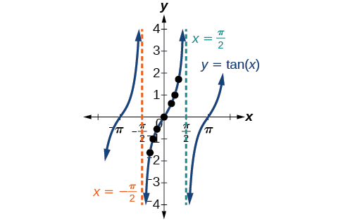
Figure 1 Graph of the tangent function
8.2.2 Graphing Variations of \(y\) = tan \(x\)
As with the sine and cosine functions, the tangent function can be described by a general equation.
\[y = A\tan(Bx)\]
We can identify horizontal and vertical stretches and compressions using values of \(A\) and \(B.\) The horizontal stretch can typically be determined from the period of the graph. With tangent graphs, it is often necessary to determine a vertical stretch using a point on the graph.
Because there are no maximum or minimum values of a tangent function, the term amplitude cannot be interpreted as it is for the sine and cosine functions. Instead, we will use the phrase stretching/compressing factor when referring to the constant \(A.\)
Graphing One Period of a Stretched or Compressed Tangent Function
We can use what we know about the properties of the tangent function to quickly sketch a graph of any stretched and/or compressed tangent function of the form \(f(x) = A\tan(Bx).\) We focus on a single period of the function including the origin, because the periodic property enables us to extend the graph to the rest of the function’s domain if we wish. Our limited domain is then the interval \(\left( {- \frac{P}{2},\frac{P}{2}} \right)\) and the graph has vertical asymptotes at \(\pm \frac{P}{2}\) where \(P = \frac{\pi}{B}.\) On \(\left( {- \frac{\pi}{2},\frac{\pi}{2}} \right),\) the graph will come up from the left asymptote at \(x = - \frac{\pi}{2},\) cross through the origin, and continue to increase as it approaches the right asymptote at \(x = \frac{\pi}{2}.\) To make the function approach the asymptotes at the correct rate, we also need to set the vertical scale by actually evaluating the function for at least one point that the graph will pass through. For example, we can use
\[f\left( \frac{P}{4} \right) = A\tan\left( {B\frac{P}{4}} \right) = A\tan\left( {B\frac{\pi}{4B}} \right) = A\]
because \(\tan\left( \frac{\pi}{4} \right) = 1.\)
Sketch a graph of one period of the function \(y = 0.5\tan\left( {\frac{\pi}{2}x} \right).\)
Solution (click to reveal)
First, we identify \(A\) and \(B.\)

Because \(A = 0.5\) and \(B = \frac{\pi}{2},\) we can find the stretching/compressing factor and period. The period is \(\frac{\pi}{\frac{\pi}{2}} = 2,\) so the asymptotes are at \(x = \pm 1.\) At a quarter period from the origin, we have
\[\begin{array}{l} {f(0.5) = 0.5\tan\left( \frac{0.5\pi}{2} \right)} \\ {= 0.5\tan\left( \frac{\pi}{4} \right)} \\ {= 0.5} \end{array}\]
This means the curve must pass through the points \(\left( {0.5,0.5} \right),\) \(\left( {0,0} \right),\) and \(\left( {- 0.5,-0.5} \right).\) The only inflection point is at the origin. Figure 2 shows the graph of one period of the function.
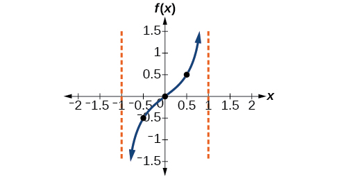
Figure 2
Sketch a graph of \(f(x) = 3\tan\left( {\frac{\pi}{6}x} \right).\)
Solution (click to reveal)
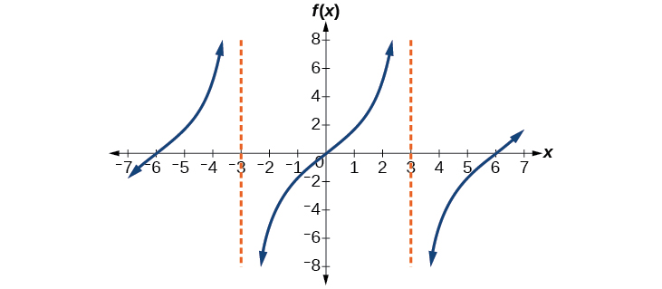
Graphing One Period of a Shifted Tangent Function
Now that we can graph a tangent function that is stretched or compressed, we will add a vertical and/or horizontal (or phase) shift. In this case, we add \(C\) and \(D\) to the general form of the tangent function.
\[f(x) = A\tan(Bx - C) + D\]
The graph of a transformed tangent function is different from the basic tangent function \(\tan\; x\) in several ways:
Graph one period of the function \(y = -2\tan(\pi x + \pi)-1.\)
Solution (click to reveal)
Step 1. The function is already written in the form \(y = A\tan\left( {Bx - C} \right) + D.\)
Step 2. \(A = -2,\) so the stretching factor is \(|A| = 2.\)
Step 3. \(B = \pi,\) so the period is \(P = \frac{\pi}{|B|} = \frac{\pi}{\pi} = 1.\)
Step 4. \(C = - \pi,\) so the phase shift is \(\frac{C}{B} = \frac{- \pi}{\pi} = -1.\)
Step 5-7. The asymptotes are at \(x = - \frac{3}{2}\) and \(x = - \frac{1}{2}\) and the three recommended reference points are \(\left( {-1.25,1} \right),\) \(\left( {-1,-1} \right),\) and \(\left( {-0.75,-3} \right).\) The graph is shown in Figure 3.
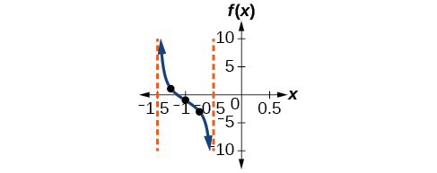
Figure 3
Note that this is a decreasing function because \(A < 0.\)
Find a formula for the function graphed in Figure 4.
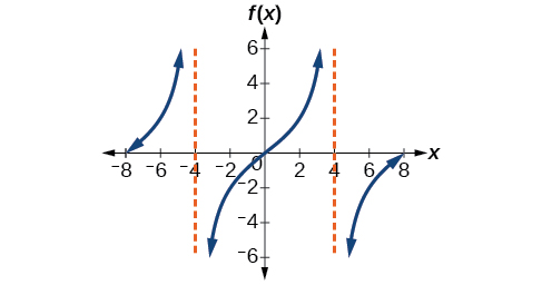
Figure 4 A stretched tangent function
Solution (click to reveal)
The graph has the shape of a tangent function.
Step 1. One cycle extends from –4 to 4, so the period is \(P = 8.\) Since \(P = \frac{\pi}{|B|},\) we have \(B = \frac{\pi}{P} = \frac{\pi}{8}.\)
Step 2. The equation must have the form \(f(x) = A\tan\left( {\frac{\pi}{8}x} \right).\)
Step 3. To find the vertical stretch \(A,\) we can use the point \(\left( {2,2} \right).\)
\[2 = A\tan\left( {\frac{\pi}{8} \cdot 2} \right) = A\tan\left( \frac{\pi}{4} \right)\]
Because \(\tan\left( \frac{\pi}{4} \right) = 1,\) \(A = 2.\)
This function would have a formula \(f(x) = 2\tan\left( {\frac{\pi}{8}x} \right).\)
Find a formula for the function in Figure 5.
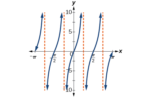
Figure 5
Solution (click to reveal)
\(g(x) = 4\tan(2x)\)
8.2.3 Analyzing the Graphs of \(y\) = sec \(x\) and \(y\) = cscx
The secant was defined by the reciprocal identity \(\sec\; x = \frac{1}{\cos\; x}.\) Notice that the function is undefined when the cosine is 0, leading to vertical asymptotes at \(\frac{\pi}{2},\) \(\frac{3\pi}{2},\) etc. Because the cosine is never more than 1 in absolute value, the secant, being the reciprocal, will never be less than 1 in absolute value.
We can graph \(y = \sec\; x\) by observing the graph of the cosine function because these two functions are reciprocals of one another. See Figure 6. The graph of the cosine is shown as a dashed orange wave so we can see the relationship. Where the graph of the cosine function decreases, the graph of the secant function increases. Where the graph of the cosine function increases, the graph of the secant function decreases. When the cosine function is zero, the secant is undefined.
The secant graph has vertical asymptotes at each value of \(x\) where the cosine graph crosses the \(x\)-axis; we show these in the graph below with dashed vertical lines, but will not show all the asymptotes explicitly on all later graphs involving the secant and cosecant.
Note that, because cosine is an even function, secant is also an even function. That is, \(\sec\left( {- x} \right) = \sec\; x.\)
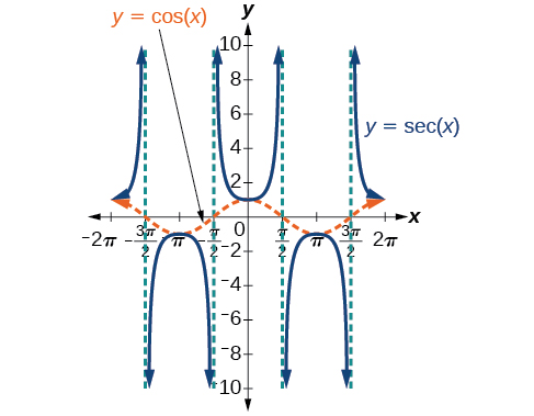
Figure 6 Graph of the secant function, \(f(x) = \sec x = \frac{1}{\cos x}\)
As we did for the tangent function, we will again refer to the constant \(|A|\) as the stretching factor, not the amplitude.
Similar to the secant, the cosecant is defined by the reciprocal identity \(\csc\; x = \frac{1}{\sin\; x}.\) Notice that the function is undefined when the sine is 0, leading to a vertical asymptote in the graph at \(0,\) \(\pi,\) etc. Since the sine is never more than 1 in absolute value, the cosecant, being the reciprocal, will never be less than 1 in absolute value.
We can graph \(y = \csc\; x\) by observing the graph of the sine function because these two functions are reciprocals of one another. See Figure 7. The graph of sine is shown as a dashed orange wave so we can see the relationship. Where the graph of the sine function decreases, the graph of the cosecant function increases. Where the graph of the sine function increases, the graph of the cosecant function decreases.
The cosecant graph has vertical asymptotes at each value of \(x\) where the sine graph crosses the \(x\)-axis; we show these in the graph below with dashed vertical lines.
Note that, since sine is an odd function, the cosecant function is also an odd function. That is, \(\csc\left( {- x} \right) = {-csc}x.\)
The graph of cosecant, which is shown in Figure 7, is similar to the graph of secant.
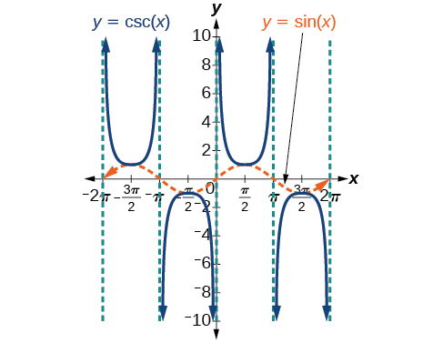
Figure 7 The graph of the cosecant function, \(f(x) = \csc x = \frac{1}{\sin x}\)
8.2.4 Graphing Variations of \(y\) = sec \(x\) and \(y\)= csc \(x\)
For shifted, compressed, and/or stretched versions of the secant and cosecant functions, we can follow similar methods to those we used for tangent and cotangent. That is, we locate the vertical asymptotes and also evaluate the functions for a few points (specifically the local extrema). If we want to graph only a single period, we can choose the interval for the period in more than one way. The procedure for secant is very similar, because the cofunction identity means that the secant graph is the same as the cosecant graph shifted half a period to the left. Vertical and phase shifts may be applied to the cosecant function in the same way as for the secant and other functions.The equations become the following.
\[y = A\sec\left( {Bx - C} \right) + D\]
\[y = A\csc\left( {Bx - C} \right) + D\]
Graph one period of \(f(x) = 2.5\sec(0.4x).\)
Solution (click to reveal)
Step 1. The given function is already written in the general form, \(y = A\sec\left( {Bx} \right).\)
Step 2. \(A = 2.5\) so the stretching factor is \(\text{2}\text{.5}\text{.}\)
Step 3. \(B = 0.4\) so \(P = \frac{2\pi}{0.4} = 5\pi.\) The period is \(5\pi\) units.
Step 4. Sketch the graph of the function \(g(x) = 2.5\cos(0.4x).\)
Step 5. Use the reciprocal relationship of the cosine and secant functions to draw the cosecant function.
Steps 6–7. Sketch two asymptotes at \(x = 1.25\pi\) and \(x = 3.75\pi.\) We can use two reference points, the local minimum at \(\left( {0,2.5} \right)\) and the local maximum at \(\left( {2.5\pi,-2.5} \right).\) Figure 8 shows the graph.
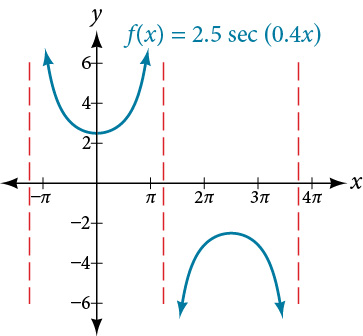
Figure 8
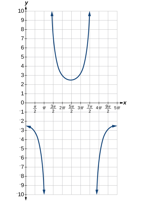
Graph one period of \(f(x) = - 2.5\sec(0.4x).\)
Solution (click to reveal)
This is a vertical reflection of the preceding graph because \(A\) is negative.
Graph one period of \(y = 4\sec\left( {\frac{\pi}{3}x - \frac{\pi}{2}} \right) + 1.\)
Solution (click to reveal)
Step 1. Express the function given in the form \(y = 4\sec\left( {\frac{\pi}{3}x - \frac{\pi}{2}} \right) + 1.\)
Step 2. The stretching/compressing factor is \(|A| = 4.\)
Step 3. The period is
\[\begin{array}{l} {\frac{2\pi}{|B|} = \frac{2\pi}{\frac{\pi}{3}}} \\ {\text{~~~~~~} = \frac{2\pi}{1} \cdot \frac{3}{\pi}} \\ {\text{~~~~~~} = 6} \end{array}\]
- Step 4. The phase shift is
\[\begin{array}{l} {\frac{C}{B} = \frac{\frac{\pi}{2}}{\frac{\pi}{3}}} \\ {\text{~~~} = \frac{\pi}{2} \cdot \frac{3}{\pi}} \\ {\text{~~~} = 1.5} \end{array}\]
Step 5. Draw the graph of \(y = A\sec(Bx),\) but shift it to the right by \(\frac{C}{B} = 1.5\) and up by \(D = 1.\)
Step 6. Sketch the vertical asymptotes, which occur at \(x = 0,x = 3,\) and \(x = 6.\) There is a local minimum at \(\left( {1.5,5} \right)\) and a local maximum at \(\left( {4.5, - 3} \right).\) Figure 9 shows the graph.
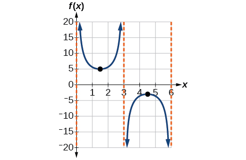
Figure 9
Graph one period of \(f(x) = - 6\sec(4x + 2) - 8.\)
Solution (click to reveal)
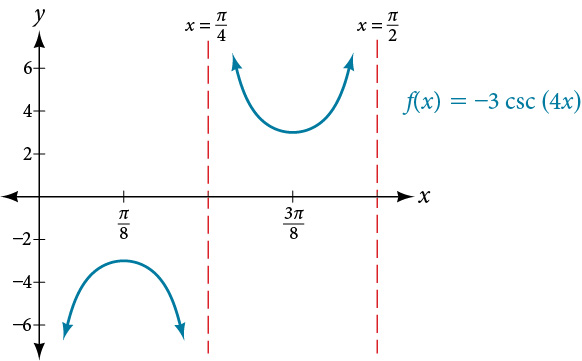
Graph one period of \(f(x) = -3\csc(4x).\)
Solution (click to reveal)
Step 1. The given function is already written in the general form, \(y = A\csc\left( {Bx} \right).\)
Step 2. \(|A| = \left| {- 3} \right| = 3,\) so the stretching factor is 3.
Step 3. \(B = 4,\) so \(P = \frac{2\pi}{4} = \frac{\pi}{2}.\) The period is \(\frac{\pi}{2}\) units.
Step 4. Sketch the graph of the function \(g(x) = -3\sin(4x).\)
Step 5. Use the reciprocal relationship of the sine and cosecant functions to draw the cosecant function.
Steps 6–7. Sketch three asymptotes at \(x = 0,\; x = \frac{\pi}{4},\) and \(x = \frac{\pi}{2}.\) We can use two reference points, the local maximum at \(\left( {\frac{\pi}{8},-3} \right)\) and the local minimum at \(\left( {\frac{3\pi}{8},3} \right).\) Figure 10 shows the graph.
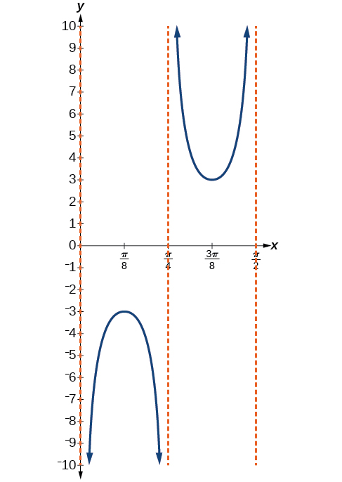
Figure 10
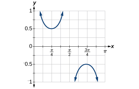
Graph one period of \(f(x) = 0.5\csc(2x).\)
Solution (click to reveal)
Sketch a graph of \(y = 2\csc\left( {\frac{\pi}{2}x} \right) + 1.\) What are the domain and range of this function?
Solution (click to reveal)
- Step 1. Express the function given in the form \(y = 2\csc\left( {\frac{\pi}{2}x} \right) + 1.\)
- Step 2. Identify the stretching/compressing factor, \(|A| = 2.\)
- Step 3. The period is \(\frac{2\pi}{|B|} = \frac{2\pi}{\frac{\pi}{2}} = \frac{2\pi}{1} \cdot \frac{2}{\pi} = 4.\)
- Step 4. The phase shift is \(\frac{0}{\frac{\pi}{2}} = 0.\)
- Step 5. Draw the graph of \(y = A\csc(Bx)\) but shift it up \(D = 1.\)
- Step 6. Sketch the vertical asymptotes, which occur at \(x = 0,x = 2,x = 4.\)
The graph for this function is shown in Figure 11.
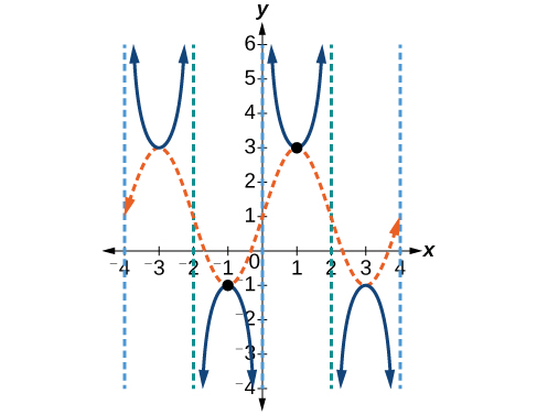
Figure 11 A transformed cosecant function
The vertical asymptotes shown on the graph mark off one period of the function, and the local extrema in this interval are shown by dots. Notice how the graph of the transformed cosecant relates to the graph of \(f(x) = 2\sin\left( {\frac{\pi}{2}x} \right) + 1,\) shown as the orange dashed wave.
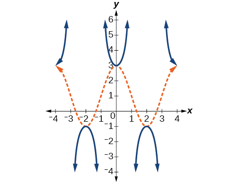
Given the graph of \(f(x) = 2\cos\left( {\frac{\pi}{2}x} \right) + 1\) shown in Figure 12, sketch the graph of \(g(x) = 2\sec\left( {\frac{\pi}{2}x} \right) + 1\) on the same axes.
![A graph of two periods of a modified cosine function. Range is [-1,3], graphed from x=-4 to x=4.](../images/CNX_Precalc_Figure_06_02_015.jpg)
Figure 12
Solution (click to reveal)
8.2.5 Analyzing the Graph of \(y\) = cot \(x\)
The last trigonometric function we need to explore is cotangent. The cotangent is defined by the reciprocal identity \(\cot\; x = \frac{1}{\tan\; x}.\) Notice that the function is undefined when the tangent function is 0, leading to a vertical asymptote in the graph at \(0,\pi,\) etc. Since the output of the tangent function is all real numbers, the output of the cotangent function is also all real numbers.
We can graph \(y = \cot\; x\) by observing the graph of the tangent function because these two functions are reciprocals of one another. See Figure 13. Where the graph of the tangent function decreases, the graph of the cotangent function increases. Where the graph of the tangent function increases, the graph of the cotangent function decreases.
The cotangent graph has vertical asymptotes at each value of \(x\) where \(\tan\; x = 0;\) we show these in the graph below with dashed lines. Since the cotangent is the reciprocal of the tangent, \(\cot\; x\) has vertical asymptotes at all values of \(x\) where \(\tan\; x = 0,\) and \(\cot\; x = 0\) at all values of \(x\) where \(\tan\; x\) has its vertical asymptotes.
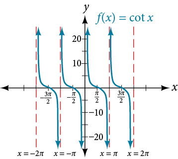
Figure 13 The cotangent function
8.2.6 Graphing Variations of \(y\) = cot \(x\)
We can transform the graph of the cotangent in much the same way as we did for the tangent. The equation becomes the following.
\[y = A\cot\left( {Bx - C} \right) + D\]
Determine the stretching factor, period, and phase shift of \(y = 3\cot(4x),\) and then sketch a graph.
Solution (click to reveal)
- Step 1. Expressing the function in the form \(f(x) = A\cot\left( {Bx} \right)\) gives \(f(x) = 3\cot\left( {4x} \right).\)
- Step 2. The stretching factor is \(|A| = 3.\)
- Step 3. The period is \(P = \frac{\pi}{4}.\)
- Step 4. Sketch the graph of \(y = 3\tan(4x).\)
- Step 5. Plot two reference points. Two such points are \(\left( {\frac{\pi}{16},3} \right)\) and \(\left( {\frac{3\pi}{16},-3} \right).\)
- Step 6. Use the reciprocal relationship to draw \(y = 3\cot(4x).\)
- Step 7. Sketch the asymptotes, \(x = 0,\; x = \frac{\pi}{4}.\)
The blue graph in Figure 14 shows \(y = 3\tan\left( {4x} \right)\) and the green graph shows \(y = 3\cot\left( {4x} \right).\)
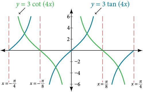
Figure 14
Sketch a graph of one period of the function \(f(x) = 4\cot\left( {\frac{\pi}{8}x - \frac{\pi}{2}} \right) - 2.\)
Solution (click to reveal)
- Step 1. The function is already written in the general form \(f(x) = A\cot\left( {Bx - C} \right) + D.\)
- Step 2. \(A = 4,\) so the stretching factor is 4.
- Step 3. \(B = \frac{\pi}{8},\) so the period is \(P = \frac{\pi}{|B|} = \frac{\pi}{\frac{\pi}{8}} = 8.\)
- Step 4. \(C = \frac{\pi}{2},\) so the phase shift is \(\frac{C}{B} = \frac{\frac{\pi}{2}}{\frac{\pi}{8}} = 4.\)
- Step 5. We draw \(f(x) = 4\tan\left( {\frac{\pi}{8}x - \frac{\pi}{2}} \right) - 2.\)
- Step 6-7. Three points we can use to guide the graph are \((6,2),(8, - 2),\) and \((10, - 6).\) We use the reciprocal relationship of tangent and cotangent to draw \(f(x) = 4\cot\left( {\frac{\pi}{8}x - \frac{\pi}{2}} \right) - 2.\)
- Step 8. The vertical asymptotes are \(x = 4\) and \(x = 12.\)
The graph is shown in Figure 15.
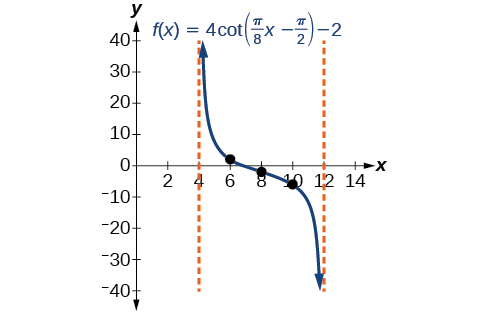
Figure 15 One period of a modified cotangent function
8.2.7 Using the Graphs of Trigonometric Functions to Solve Real-World Problems
Many real-world scenarios represent periodic functions and may be modeled by trigonometric functions. As an example, let’s return to the scenario from the section opener. Have you ever observed the beam formed by the rotating light on a fire truck and wondered about the movement of the light beam itself across the wall? The periodic behavior of the distance the light shines as a function of time is obvious, but how do we determine the distance? We can use the tangent function.
Suppose the function \(y = 5\tan\left( {\frac{\pi}{4}t} \right)\) marks the distance in the movement of a light beam from the top of a police car across a wall where \(t\) is the time in seconds and \(y\) is the distance in feet from a point on the wall directly across from the police car.
ⓐ Find and interpret the stretching factor and period.
ⓑ Graph on the interval \(\left\lbrack {0,5} \right\rbrack.\)
ⓒ Evaluate \(f(1)\) and discuss the function’s value at that input.
Solution (click to reveal)
ⓐ We know from the general form of \(y = A\tan\left( {Bt} \right)\) that \(|A|\) is the stretching factor and \(\frac{\pi}{B}\) is the period.

Figure 16
The vertical stretch factor of 5 means that the beam will have moved 5 feet in the one-quarter period before or after the half-period mark. This corresponds to the y-value of the standard tangent function being 1 at one-quarter of the period away from the center of the period, multiplied by the stretching factor of 5. The period is \(\frac{\pi}{\frac{\pi}{4}} = \frac{\pi}{1} \cdot \frac{4}{\pi} = 4.\) This means that every 4 seconds, the beam of light sweeps the wall. The distance from the spot across from the police car grows larger as the police car approaches.
ⓑ To graph the function, we draw an asymptote at \(t = 2\) and use the stretching factor and period. See Figure 17
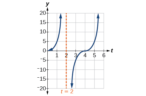
Figure 17
ⓒ period: \(f(1) = 5\tan\left( {\frac{\pi}{4}(1)} \right) = 5(1) = 5;\) after 1 second, the beam of has moved 5 ft from the spot across from the police car.
Section Exercises
Verbal
1. Explain how the graph of the sine function can be used to graph \(y = \csc\; x.\)
Solution (click to reveal)
Since \(y = \csc\; x\) is the reciprocal function of \(y = \sin\; x,\) you can plot the reciprocal of the coordinates on the graph of \(y = \sin\; x\) to obtain the \(y\)-coordinates of \(y = \csc\; x.\) The \(x\)-intercepts of the graph \(y = \sin\; x\) are the vertical asymptotes for the graph of \(y = \csc\; x.\)
2. How can the graph of \(y = \cos\; x\) be used to construct the graph of \(y = \sec\; x?\)
3. Explain why the period of \(\tan\; x\) is equal to \(\pi.\)
Solution (click to reveal)
Answers will vary. Using the unit circle, one can show that \(\tan\left( {x + \pi} \right) = \tan\; x.\)
4. Why are there no intercepts on the graph of \(y = \csc\; x?\)
5. How does the period of \(y = \csc\; x\) compare with the period of \(y = \sin\; x?\)
Solution (click to reveal)
The period is the same: \(2\pi.\)
Algebraic
For the following exercises, match each trigonometric function with one of the following graphs.
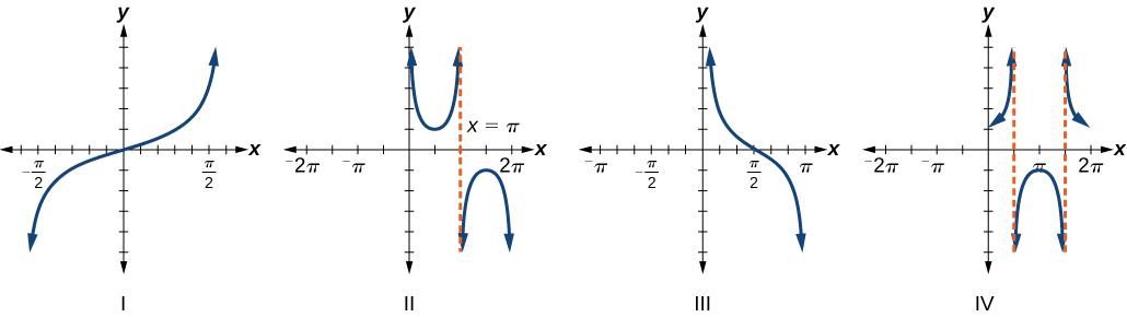
Figure 18
6. \(f(x) = \tan\; x\)
7. \(f(x) = \sec\; x\)
Solution (click to reveal)
IV
8. \(f(x) = \csc\; x\)
9. \(f(x) = \cot\; x\)
Solution (click to reveal)
III
For the following exercises, find the period and horizontal shift of each of the functions.
10. \(f(x) = 2\tan\left( {4x - 32} \right)\)
11. \(h(x) = 2\sec\left( {\frac{\pi}{4}\left( {x + 1} \right)} \right)\)
Solution (click to reveal)
period: 8; horizontal shift: 1 unit to left
12. \(m(x) = 6\csc\left( {\frac{\pi}{3}x + \pi} \right)\)
For the following exercises, evaluate the transformed functions.
13. If \(\tan\; x = -1.5,\) find \(\tan\left( {- x} \right).\)
Solution (click to reveal)
1.5
14. If \(\sec\; x = 2,\) find \(\sec\left( {- x} \right).\)
15. If \(\csc\; x = -5,\) find \(\csc\left( {- x} \right).\)
Solution (click to reveal)
5
16. If \(x\sin\; x = 2,\) find \(\left( {- x} \right)\sin\left( {- x} \right).\)
For the following exercises, rewrite each expression such that the argument \(x\) is positive.
17. \(\cot\left( {- x} \right)\cos\left( {- x} \right) + \sin\left( {- x} \right)\)
Solution (click to reveal)
\(- \cot x\cos x - \sin x\)
18. \(\cos\left( {- x} \right) + \tan\left( {- x} \right)\sin\left( {- x} \right)\)
Graphical
For the following exercises, sketch two periods of the graph for each of the following functions. Identify the stretching factor, period, and asymptotes.
19. \(f(x) = 2\tan\left( {4x - 32} \right)\)
Solution (click to reveal)
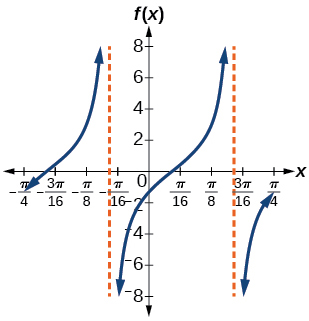
stretching factor: 2; period: \(\frac{\pi}{4};\) asymptotes: \(x = \frac{1}{4}\left( {\frac{\pi}{2} + \pi k} \right) + 8,\text{~where~}k\text{~is~an~integer}\)
20. \(h(x) = 2\sec\left( {\frac{\pi}{4}\left( {x + 1} \right)} \right)\)
21. \(m(x) = 6\csc\left( {\frac{\pi}{3}x + \pi} \right)\)
Solution (click to reveal)
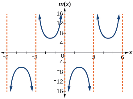
stretching factor: 6; period: 6; asymptotes: \(x = 3k,\text{~where~}k\text{~is~an~integer}\)
22. \(j(x) = \tan\left( {\frac{\pi}{2}x} \right)\)
23. \(p(x) = \tan\left( {x - \frac{\pi}{2}} \right)\)
Solution (click to reveal)
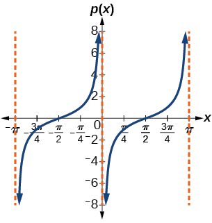
stretching factor: 1; period: \(\pi;\) asymptotes: \(x = \pi k,\text{~where~}k\text{~is~an~integer}\)
24. \(f(x) = 4\tan(x)\)
25. \(f(x) = \tan\left( {x + \frac{\pi}{4}} \right)\)
Solution (click to reveal)
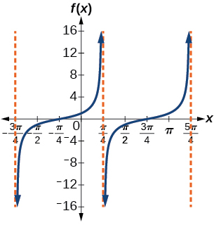
Stretching factor: 1; period: \(\pi;\) asymptotes: \(x = \frac{\pi}{4} + \pi k,\text{~where~}k\text{~is~an~integer}\)
26. \(f(x) = \pi\tan\left( {\pi x - \pi} \right) - \pi\)
27. \(f(x) = 2\csc(x)\)
Solution (click to reveal)
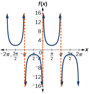
stretching factor: 2; period: \(2\pi;\) asymptotes: \(x = \pi k,\text{~where~}k\text{~is~an~integer}\)
28. \(f(x) = - \frac{1}{4}\csc(x)\)
29. \(f(x) = 4\sec\left( {3x} \right)\)
Solution (click to reveal)
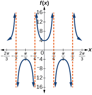
stretching factor: 4; period: \(\frac{2\pi}{3};\) asymptotes: \(x = \frac{\pi}{6}k,\text{~where~}k\text{~is~an~odd~integer}\)
30. \(f(x) = - 3\cot\left( {2x} \right)\)
31. \(f(x) = 7\sec\left( {5x} \right)\)
Solution (click to reveal)
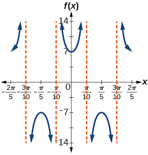
stretching factor: 7; period: \(\frac{2\pi}{5};\) asymptotes: \(x = \frac{\pi}{10}k,\text{~where~}k\text{~is~an~odd~integer}\)
32. \(f(x) = \frac{9}{10}\csc\left( {\pi x} \right)\)
33. \(f(x) = 2\csc\left( {x + \frac{\pi}{4}} \right) - 1\)
Solution (click to reveal)
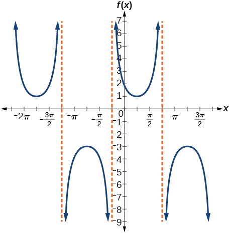
stretching factor: 2; period: \(2\pi;\) asymptotes: \(x = - \frac{\pi}{4} + \pi k,\text{~where~}k\text{~is~an~integer}\)
34. \(f(x) = - \sec\left( {x - \frac{\pi}{3}} \right) - 2\)
35. \(f(x) = \frac{7}{5}\csc\left( {x - \frac{\pi}{4}} \right)\)
Solution (click to reveal)
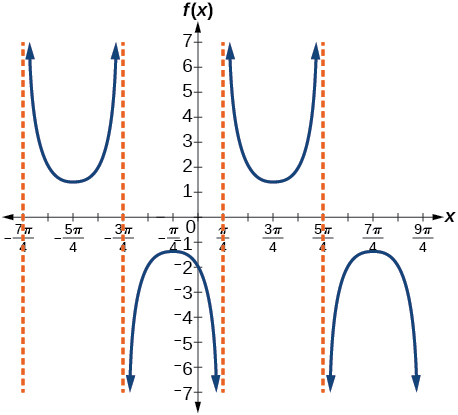
stretching factor: \(\frac{7}{5};\) period: \(2\pi;\) asymptotes: \(x = \frac{\pi}{4} + \pi k,\text{~where~}k\text{~is~an~integer}\)
36. \(f(x) = 5\left( {\cot\left( {x + \frac{\pi}{2}} \right) - 3} \right)\)
For the following exercises, find and graph two periods of the periodic function with the given stretching factor, \(|A|,\) period, and phase shift.
37. A tangent curve, \(A = 1,\) period of \(\frac{\pi}{3};\) and phase shift \(\left( {h,\; k} \right) = \left( {\frac{\pi}{4},2} \right)\)
Solution (click to reveal)
\(y = \tan\left( {3\left( {x - \frac{\pi}{4}} \right)} \right) + 2\)
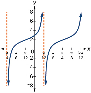
38. A tangent curve, \(A = -2,\) period of \(\frac{\pi}{4},\) and phase shift \(\left( {h,\; k} \right) = \left( {- \frac{\pi}{4},\;-2} \right)\)
For the following exercises, find an equation for the graph of each function.
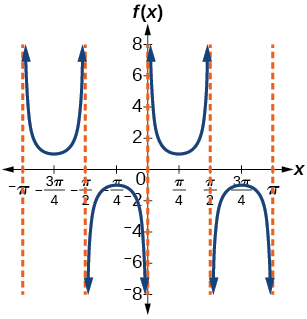
39.
Solution (click to reveal)
\(f(x) = \csc\left( {2x} \right)\)
40.
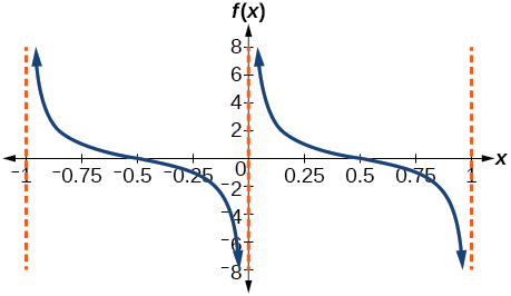
41.
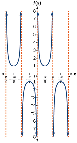
Solution (click to reveal)
\(f(x) = \csc\left( {4x} \right)\)
42.
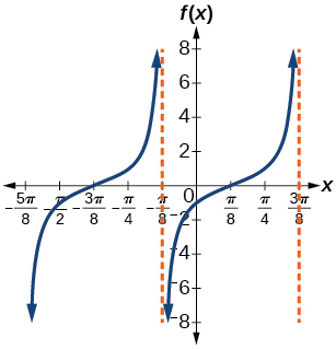
43.
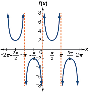
Solution (click to reveal)
\(f(x) = 2\csc x\)
44.
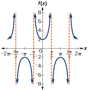
45.
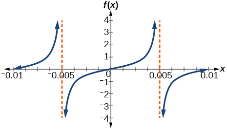
Solution (click to reveal)
\(f(x) = \frac{1}{2}\tan(100\pi x)\)
Technology
For the following exercises, use a graphing calculator to graph two periods of the given function. Note: most graphing calculators do not have a cosecant button; therefore, you will need to input \(\csc\; x\) as \(\frac{1}{\sin\; x}.\)
46. \(f(x) = \left| {\csc(x)} \right|\)
47. \(f(x) = \left| {\cot(x)} \right|\)
Solution (click to reveal)
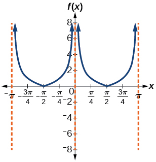
48. \(f(x) = 2^{\csc{(x)}}\)
49. \(f(x) = \frac{\csc(x)}{\sec(x)}\)
Solution (click to reveal)
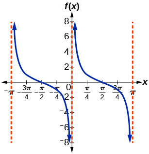
50. Graph \(f(x) = 1 + \sec^{2}(x) - \tan^{2}(x).\) What is the function shown in the graph?
51. \(f(x) = \sec\left( {0.001x} \right)\)
Solution (click to reveal)
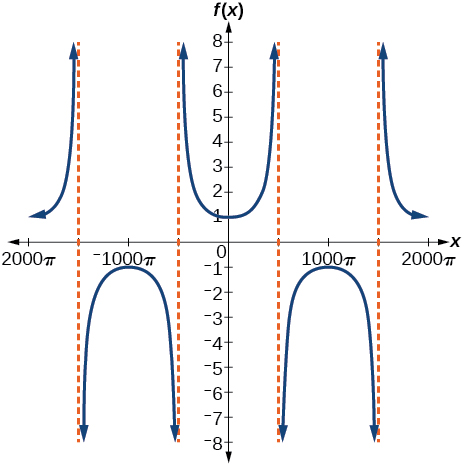
52. \(f(x) = \cot\left( {100\pi x} \right)\)
53. \(f(x) = \sin^{2}x + \cos^{2}x\)
Solution (click to reveal)
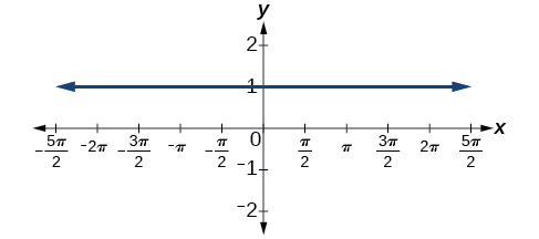
Real-World Applications
54. The function \(f(x) = 20\tan\left( {\frac{\pi}{10}x} \right)\) marks the distance in the movement of a light beam from a police car across a wall for time \(x,\) in seconds, and distance \(f(x),\) in feet.
ⓐ Graph on the interval \(\left\lbrack {0,\; 5} \right\rbrack.\)
ⓑ Find and interpret the stretching factor, period, and asymptote.
ⓒ Evaluate \(f(1)\) and \(f(2.5)\) and discuss the function’s values at those inputs.
55. Standing on the shore of a lake, a fisherman sights a boat far in the distance to his left. Let \(x,\) measured in radians, be the angle formed by the line of sight to the ship and a line due north from his position. Assume due north is 0 and \(x\) is measured negative to the left and positive to the right. (See Figure 19.) The boat travels from due west to due east and, ignoring the curvature of the Earth, the distance \(d(x),\) in kilometers, from the fisherman to the boat is given by the function \(d(x) = 1.5\sec(x).\)
ⓐ What is a reasonable domain for \(d(x)?\)
ⓑ Graph \(d(x)\) on this domain.
ⓒ Find and discuss the meaning of any vertical asymptotes on the graph of \(d(x).\)
ⓓ Calculate and interpret \(d\left( {- \frac{\pi}{3}} \right).\) Round to the second decimal place.
ⓔ Calculate and interpret \(d\left( \frac{\pi}{6} \right).\) Round to the second decimal place.
ⓕ What is the minimum distance between the fisherman and the boat? When does this occur?
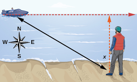
Figure 19
Solution (click to reveal)
ⓐ \(\left( {- \frac{\pi}{2},\;\frac{\pi}{2}} \right);\)
ⓑ
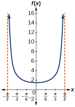
ⓒ \(x = - \frac{\pi}{2}\) and \(x = \frac{\pi}{2};\) the distance grows without bound as \(|x|\) approaches \(\frac{\pi}{2}\) —i.e., at right angles to the line representing due north, the boat would be so far away, the fisherman could not see it;
ⓓ 3; when \(x = - \frac{\pi}{3},\) the boat is 3 km away;
ⓔ 1.73; when \(x = \frac{\pi}{6},\) the boat is about 1.73 km away;
ⓕ 1.5 km; when \(x = 0\)
56. A laser rangefinder is locked on a comet approaching Earth. The distance \(g(x),\) in kilometers, of the comet after \(x\) days, for \(x\) in the interval 0 to 30 days, is given by \(g(x) = 250{,}000\csc\left( {\frac{\pi}{30}x} \right).\)
ⓐ Graph \(g(x)\) on the interval \(\left\lbrack {0,\; 30} \right\rbrack.\)
ⓑ Evaluate \(g(5)\) and interpret the information.
ⓒ What is the minimum distance between the comet and Earth? When does this occur? To which constant in the equation does this correspond?
ⓓ Find and discuss the meaning of any vertical asymptotes.
57. A video camera is focused on a rocket on a launching pad 2 miles from the camera. The angle of elevation from the ground to the rocket after \(x\) seconds is \(\frac{\pi}{120}x.\)
ⓐ Write a function expressing the altitude \(h(x),\) in miles, of the rocket above the ground after \(x\) seconds. Ignore the curvature of the Earth.
ⓑ Graph \(h(x)\) on the interval \(\left( {0,\mspace{9mu} 60} \right).\)
ⓒ Evaluate and interpret the values \(h(0)\) and \(h(30).\)
ⓓ What happens to the values of \(h(x)\) as \(x\) approaches 60 seconds? Interpret the meaning of this in terms of the problem.
Solution (click to reveal)
ⓐ \(h(x) = 2\tan\left( {\frac{\pi}{120}x} \right);\)
ⓑ
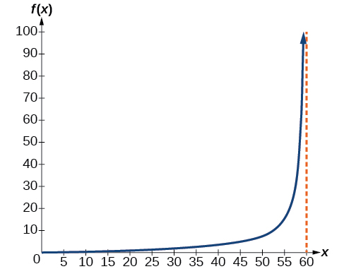
ⓒ \(h(0) = 0:\) after 0 seconds, the rocket is 0 mi above the ground; \(h(30) = 2:\) after 30 seconds, the rockets is 2 mi high;
ⓓ As \(x\) approaches 60 seconds, the values of \(h(x)\) grow increasingly large. The distance to the rocket is growing so large that the camera can no longer track it.