3.3 Rates of Change and Behavior of Graphs

NoteLearning Objectives

In this section, you will:

• Find the average rate of change of a function.
• Use a graph to determine where a function is increasing, decreasing, or constant.
• Use a graph to locate local maxima and local minima.
• Use a graph to locate the absolute maximum and absolute minimum.

Gasoline costs have experienced some wild fluctuations over the last several decades. Table 1 lists the average cost, in dollars, of a gallon of gasoline for the years 2005–2012. The cost of gasoline can be considered as a function of year.

\(y\)	2005	2006	2007	2008	2009	2010	2011	2012
\(C(y)\)	2.31	2.62	2.84	3.30	2.41	2.84	3.58	3.68

Table 1

If we were interested only in how the gasoline prices changed between 2005 and 2012, we could compute that the cost per gallon had increased from $2.31 to $3.68, an increase of $1.37. While this is interesting, it might be more useful to look at how much the price changed per year. In this section, we will investigate changes such as these.

3.3.1 Finding the Average Rate of Change of a Function

The price change per year is a rate of change because it describes how an output quantity changes relative to the change in the input quantity. We can see that the price of gasoline in Table 1 did not change by the same amount each year, so the rate of change was not constant. If we use only the beginning and ending data, we would be finding the average rate of change over the specified period of time. To find the average rate of change, we divide the change in the output value by the change in the input value.

\[\begin{array}{ccl} \text{Average~rate~of~change} & = & \frac{\text{Change~in~output}}{\text{Change~in~input}} \\ & = & \frac{\Delta y}{\Delta x} \\ & = & \frac{y_{2} - y_{1}}{x_{2} - x_{1}} \\ & = & \frac{f\left( x_{2} \right) - f\left( x_{1} \right)}{x_{2} - x_{1}} \end{array}\]

The Greek letter \(\text{Δ}\) (delta) signifies the change in a quantity; we read the ratio as “delta-\(y\) over delta-\(x\)” or “the change in \(y\) divided by the change in \(x.\)” Occasionally we write \(\text{Δ}f\) instead of \(\text{Δ}y,\) which still represents the change in the function’s output value resulting from a change to its input value. It does not mean we are changing the function into some other function.

In our example, the gasoline price increased by $1.37 from 2005 to 2012. Over 7 years, the average rate of change was

\[\frac{\text{Δ}y}{\text{Δ}x} = \frac{\text{\$}1.37}{\text{7~years}} \approx 0.196\mspace{9mu}\text{dollars~per~year}\]

On average, the price of gas increased by about 19.6¢ each year.

Other examples of rates of change include:

• A population of rats increasing by 40 rats per week
• A car traveling 68 miles per hour (distance traveled changes by 68 miles each hour as time passes)
• A car driving 27 miles per gallon (distance traveled changes by 27 miles for each gallon)
• The current through an electrical circuit increasing by 0.125 amperes for every volt of increased voltage
• The amount of money in a college account decreasing by $4,000 per quarter

NoteRate of Change

A rate of change describes how an output quantity changes relative to the change in the input quantity. The units on a rate of change are “output units per input units.”

The average rate of change between two input values is the total change of the function values (output values) divided by the change in the input values.

\[\frac{\Delta y}{\Delta x} = \frac{f\left( x_{2} \right) - f\left( x_{1} \right)}{x_{2} - x_{1}}\]

ImportantHow To

Given the value of a function at different points, calculate the average rate of change of a function for the interval between two values \(x_{1}\) and \(x_{2}.\)

1. Calculate the difference \(y_{2} - y_{1} = \text{Δ}y.\)
2. Calculate the difference \(x_{2} - x_{1} = \text{Δ}x.\)
3. Find the ratio \(\frac{\text{Δ}y}{\text{Δ}x}.\)

TipExample 1 — Computing an Average Rate of Change

Using the data in Table 1, find the average rate of change of the price of gasoline between 2007 and 2009.

Solution (click to reveal)

In 2007, the price of gasoline was $2.84. In 2009, the cost was $2.41. The average rate of change is

\[\begin{array}{ccl} \frac{\Delta y}{\Delta x} & = & \frac{y_{2} - y_{1}}{x_{2} - x_{1}} \\ & = & \frac{\$ 2.41 - \$ 2.84}{2009 - 2007} \\ & = & \frac{- \$ 0.43}{2\mspace{9mu}\text{years}} \\ & = & {- \$ 0.22\mspace{9mu}\text{per~year}} \end{array}\]

Note that a decrease is expressed by a negative change or “negative increase.” A rate of change is negative when the output decreases as the input increases or when the output increases as the input decreases.

WarningTry It #1

Using the data in Table 1, find the average rate of change between 2005 and 2010.

Solution (click to reveal)

\(\frac{\$ 2.84 - \$ 2.31}{5\mspace{9mu}\text{years}} = \frac{\$ 0.53}{5\mspace{9mu}\text{years}} = \$ 0.106\) per year.

TipExample 2 — Computing Average Rate of Change from a Graph

Given the function \(g(t)\) shown in Figure 1, find the average rate of change on the interval \(\left\lbrack {- 1,2} \right\rbrack.\)

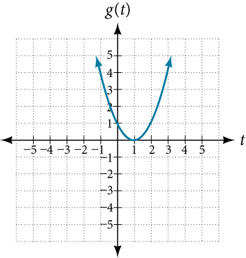
Figure 1

Solution (click to reveal)

At \(t = - 1,\) Figure 2 shows \(g(-1) = 4.\) At \(t = 2,\) the graph shows \(g(2) = 1.\)

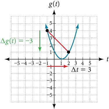
Figure 2

The horizontal change \(\text{Δ}t = 3\) is shown by the red arrow, and the vertical change \(\text{Δ}g(t) = - 3\) is shown by the turquoise arrow. The average rate of change is shown by the slope of the orange line segment. The output changes by –3 while the input changes by 3, giving an average rate of change of

\[\frac{1 - 4}{2 - \left( {- 1} \right)} = \frac{- 3}{3} = -1\]

Note that the order we choose is very important. If, for example, we use \(\frac{y_{2} - y_{1}}{x_{1} - x_{2}},\) we will not get the correct answer. Decide which point will be 1 and which point will be 2, and keep the coordinates fixed as \(\left( {x_{1},y_{1}} \right)\) and \(\left( {x_{2},y_{2}} \right).\)

TipExample 3 — Computing Average Rate of Change from a Table

After picking up a friend who lives 10 miles away and leaving on a trip, Anna records her distance from home over time. The values are shown in Table 2. Find her average speed over the first 6 hours.

\(t\) (hours)	0	1	2	3	4	5	6	7
\(D\)(\(t\)) (miles)	10	55	90	153	214	240	292	300

Table 2

Solution (click to reveal)

Here, the average speed is the average rate of change. She traveled 282 miles in 6 hours.

\[\begin{array}{ccl} \frac{292 - 10}{6 - 0} & = & \frac{282}{6} \\ & = & 47 \end{array}\]

The average speed is 47 miles per hour.

Because the speed is not constant, the average speed depends on the interval chosen. For the interval [2,3], the average speed is 63 miles per hour.

TipExample 4 — Computing Average Rate of Change for a Function Expressed as a Formula

Compute the average rate of change of \(f(x) = x^{2} - \frac{1}{x}\) on the interval \(\text{[2,}\mspace{9mu}\text{4].}\)

Solution (click to reveal)

We can start by computing the function values at each endpoint of the interval.

\[\begin{array}{cclccl} {f(2)} & = & {2^{2} - \frac{1}{2}} & {\qquad{f(4)}} & = & {4^{2} - \frac{1}{4}} \\ & = & {4 - \frac{1}{2}} & & = & {16 - \frac{1}{4}} \\ & = & \frac{7}{2} & & = & \frac{63}{4} \end{array}\]

Now we compute the average rate of change.

\[\begin{array}{ccl} \text{Average~rate~of~change} & = & \frac{f(4) - f(2)}{4 - 2} \\ & = & \frac{\frac{63}{4} - \frac{7}{2}}{4 - 2} \\ & = & \frac{\frac{49}{4}}{2} \\ & = & \frac{49}{8} \end{array}\]

WarningTry It #2

Find the average rate of change of \(f(x) = x - 2\sqrt{x}\) on the interval \(\lbrack 1,\mspace{9mu} 9\rbrack.\)

Solution (click to reveal)

\(\frac{1}{2}\)

TipExample 5 — Finding the Average Rate of Change of a Force

The electrostatic force \(F,\) measured in newtons, between two charged particles can be related to the distance between the particles \(d,\) in centimeters, by the formula \(F(d) = \frac{2}{d^{2}}.\) Find the average rate of change of force if the distance between the particles is increased from 2 cm to 6 cm.

Solution (click to reveal)

We are computing the average rate of change of \(F(d) = \frac{2}{d^{2}}\) on the interval \(\lbrack 2,6\rbrack.\)

\[\begin{array}{cclc} \text{Average~rate~of~change} & = & {\mspace{9mu}\frac{F(6) - F(2)}{6 - 2}} & \\ & = & \frac{\frac{2}{6^{2}} - \frac{2}{2^{2}}}{6 - 2} & {\text{Simplify}.} \\ & = & \frac{\frac{2}{36} - \frac{2}{4}}{4} & \\ & = & \frac{- \frac{16}{36}}{4} & {\text{Combine~numerator~terms}.} \\ & = & {- \frac{1}{9}} & \text{Simplify} \end{array}\]

The average rate of change is \(- \frac{1}{9}\) newton per centimeter.

TipExample 6 — Finding an Average Rate of Change as an Expression

Find the average rate of change of \(g(t) = t^{2} + 3t + 1\) on the interval \(\lbrack 0,\mspace{9mu} a\rbrack.\) The answer will be an expression involving \(a\) in simplest form.

Solution (click to reveal)

We use the average rate of change formula.

\[\begin{array}{cclc} \text{Average~rate~of~change} & = & \frac{g(a) - g(0)}{a - 0} & {\text{Evaluate}.} \\ & = & \frac{\left( a^{2} + 3a + 1 \right) - \left( 0^{2} + 3(0) + 1 \right)}{a - 0} & {\text{Simplify}.} \\ & = & \frac{a^{2} + 3a + 1 - 1}{a} & {\text{Simplify~and~factor}.} \\ & = & \frac{a(a + 3)}{a} & {\text{Divide~by~the~common~factor~}a.} \\ & = & {a + 3} & \end{array}\]

This result tells us the average rate of change in terms of \(a\) between \(t = 0\) and any other point \(t = a.\) For example, on the interval \(\lbrack 0,5\rbrack,\) the average rate of change would be \(5 + 3 = 8.\)

WarningTry It #3

Find the average rate of change of \(f(x) = x^{2} + 2x - 8\) on the interval \(\lbrack 5,a\rbrack\) in simplest forms in terms of \(a.\)

Solution (click to reveal)

\(a + 7\)

3.3.2 Using a Graph to Determine Where a Function is Increasing, Decreasing, or Constant

As part of exploring how functions change, we can identify intervals over which the function is changing in specific ways. We say that a function is increasing on an interval if the function values increase as the input values increase within that interval. Similarly, a function is decreasing on an interval if the function values decrease as the input values increase over that interval. The average rate of change of an increasing function is positive, and the average rate of change of a decreasing function is negative. Figure 3 shows examples of increasing and decreasing intervals on a function.

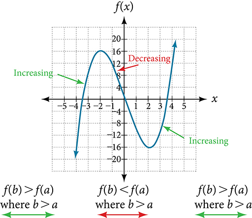
Figure 3 The function \(f(x) = x^{3} - 12x\) is increasing on \(\left( {- \infty\text{,}\mspace{9mu} - \text{2}} \right){\cup^{}}^{}\left( {2,\mspace{9mu}\infty} \right)\) and is decreasing on \(( - 2\text{,}\mspace{9mu} 2).\)

While some functions are increasing (or decreasing) over their entire domain, many others are not. A value of the input where a function changes from increasing to decreasing (as we go from left to right, that is, as the input variable increases) is the location of a local maximum. The function value at that point is the local maximum. If a function has more than one, we say it has local maxima. Similarly, a value of the input where a function changes from decreasing to increasing as the input variable increases is the location of a local minimum. The function value at that point is the local minimum. The plural form is “local minima.” Together, local maxima and minima are called local extrema, or local extreme values, of the function. (The singular form is “extremum.”) Often, the term local is replaced by the term relative. In this text, we will use the term local.

Clearly, a function is neither increasing nor decreasing on an interval where it is constant. A function is also neither increasing nor decreasing at extrema. Note that we have to speak of local extrema, because any given local extremum as defined here is not necessarily the highest maximum or lowest minimum in the function’s entire domain.

For the function whose graph is shown in Figure 4, the local maximum is 16, and it occurs at \(x = -2.\) The local minimum is \(-16\) and it occurs at \(x = 2.\)

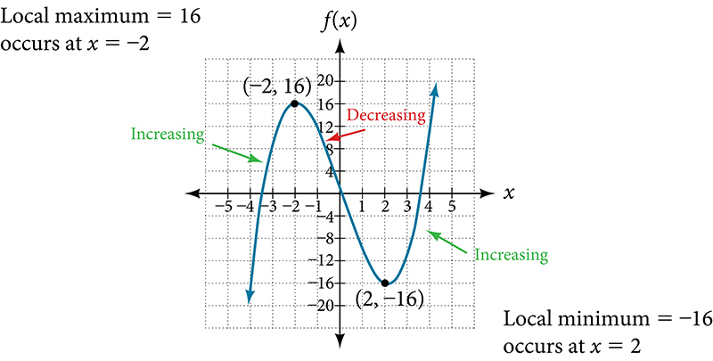
Figure 4

To locate the local maxima and minima from a graph, we need to observe the graph to determine where the graph attains its highest and lowest points, respectively, within an open interval. Like the summit of a roller coaster, the graph of a function is higher at a local maximum than at nearby points on both sides. The graph will also be lower at a local minimum than at neighboring points. Figure 5 illustrates these ideas for a local maximum.

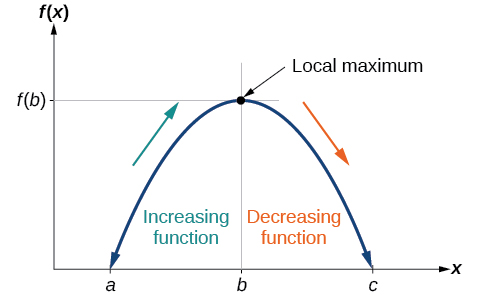
Figure 5 Definition of a local maximum

These observations lead us to a formal definition of local extrema.

NoteLocal Minima and Local Maxima

A function \(f\) is an increasing function on an open interval if \(f(b) > f(a)\) for any two input values \(a\) and \(b\) in the given interval where \(b > a.\)

A function \(f\) is a decreasing function on an open interval if \(f(b) < f(a)\) for any two input values \(a\) and \(b\) in the given interval where \(b > a.\)

A function \(f\) has a local maximum at \(x = b\) if there exists an interval \((a,c)\) with \(a < b < c\) such that, for any \(x\) in the interval \(\left( {a,c} \right),\) \(f(x) \leq f(b).\) Likewise, \(f\) has a local minimum at \(x = b\) if there exists an interval \((a,c)\) with \(a < b < c\) such that, for any \(x\) in the interval \(\left( {a,c} \right),\) \(f(x) \geq f(b).\)

TipExample 7 — Finding Increasing and Decreasing Intervals on a Graph

Given the function \(p(t)\) in Figure 6, identify the intervals on which the function appears to be increasing.

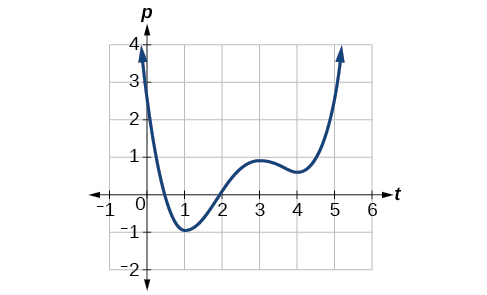
Figure 6

Solution (click to reveal)

We see that the function is not constant on any interval. The function is increasing where it slants upward as we move to the right and decreasing where it slants downward as we move to the right. The function appears to be increasing from \(t = 1\) to \(t = 3\) and from \(t = 4\) on.

In interval notation, we would say the function appears to be increasing on the interval (1,3) and the interval \((4,\infty).\)

Notice in this example that we used open intervals (intervals that do not include the endpoints), because the function is neither increasing nor decreasing at \(t = 1\) , \(t = 3\) , and \(t = 4\) . These points are the local extrema (two minima and a maximum).

TipExample 8 — Finding Local Extrema from a Graph

Graph the function \(f(x) = \frac{2}{x} + \frac{x}{3}.\) Then use the graph to estimate the local extrema of the function and to determine the intervals on which the function is increasing.

Solution (click to reveal)

Using technology, we find that the graph of the function looks like that in Figure 7. It appears there is a low point, or local minimum, between \(x = 2\) and \(x = 3,\) and a mirror-image high point, or local maximum, somewhere between \(x = -3\) and \(x = -2.\)

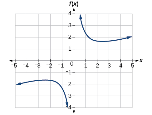
Figure 7

Most graphing calculators and graphing utilities can estimate the location of maxima and minima. Figure 8 provides screen images from two different technologies, showing the estimate for the local maximum and minimum.

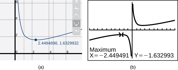
Figure 8

Based on these estimates, the function is increasing on the interval \(( - \infty\text{,} - \text{2}\text{.449)}\) and \((2.449\text{,}\infty).\) Notice that, while we expect the extrema to be symmetric, the two different technologies agree only up to four decimals due to the differing approximation algorithms used by each. (The exact location of the extrema is at \(\pm \sqrt{6},\) but determining this requires calculus.)

WarningTry It #4

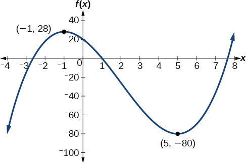
Graph the function \(f(x) = x^{3} - 6x^{2} - 15x + 20\) to estimate the local extrema of the function. Use these to determine the intervals on which the function is increasing and decreasing.

Solution (click to reveal)

The local maximum appears to occur at \(( - 1,28),\) and the local minimum occurs at \((5, - 80).\) The function is increasing on \(( - \infty, - 1) \cup (5,\infty)\) and decreasing on \(( - 1,5).\)

TipExample 9 — Finding Local Maxima and Minima from a Graph

For the function \(f\) whose graph is shown in Figure 9, find all local maxima and minima.

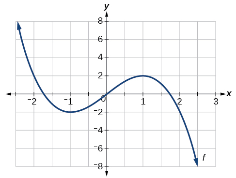
Figure 9

Solution (click to reveal)

Observe the graph of \(f.\) The graph attains a local maximum at \(x = 1\) because it is the highest point in an open interval around \(x = 1.\) The local maximum is the \(y\) -coordinate at \(x = 1,\) which is \(2.\)

The graph attains a local minimum at \(x = -1\) because it is the lowest point in an open interval around \(x = -1.\) The local minimum is the \(y\)-coordinate at \(x = -1,\) which is \(-2.\)

3.3.3 Analyzing the Toolkit Functions for Increasing or Decreasing Intervals

We will now return to our toolkit functions and discuss their graphical behavior in Figure 10, Figure 11, and Figure 12.

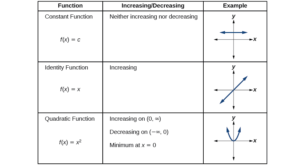
Figure 10

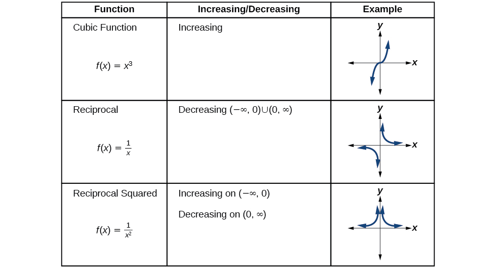
Figure 11

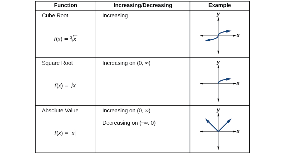
Figure 12

3.3.4 Use A Graph to Locate the Absolute Maximum and Absolute Minimum

There is a difference between locating the highest and lowest points on a graph in a region around an open interval (locally) and locating the highest and lowest points on the graph for the entire domain. The \(y\text{-}\) coordinates (output) at the highest and lowest points are called the absolute maximum andabsolute minimum, respectively.

To locate absolute maxima and minima from a graph, we need to observe the graph to determine where the graph attains it highest and lowest points on the domain of the function. See Figure 13.

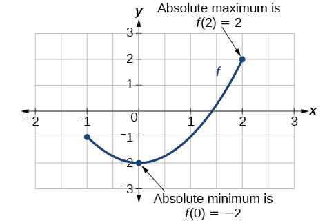
Figure 13

Not every function has an absolute maximum or minimum value. The toolkit function \(f(x) = x^{3}\) is one such function.

NoteAbsolute Maxima and Minima

The absolute maximum of \(f\) at \(x = c\) is \(f(c)\) where \(f(c) \geq f(x)\) for all \(x\) in the domain of \(f.\)

The absolute minimum of \(f\) at \(x = d\) is \(f(d)\) where \(f(d) \leq f(x)\) for all \(x\) in the domain of \(f.\)

TipExample 10 — Finding Absolute Maxima and Minima from a Graph

For the function \(f\) shown in Figure 14, find all absolute maxima and minima.

Figure 14

Solution (click to reveal)

Observe the graph of \(f.\) The graph attains an absolute maximum in two locations, \(x = -2\) and \(x = 2,\) because at these locations, the graph attains its highest point on the domain of the function. The absolute maximum is the \(y\)-coordinate at \(x = -2\) and \(x = 2,\) which is \(16.\)

The graph attains an absolute minimum at \(x = 3,\) because it is the lowest point on the domain of the function’s graph. The absolute minimum is the \(y\)-coordinate at \(x = 3,\) which is \(-10.\)

NoteMedia

Access this online resource for additional instruction and practice with rates of change.

• Average Rate of Change

Section Exercises

Verbal

1. Can the average rate of change of a function be constant?

Solution (click to reveal)

Yes, the average rate of change of all linear functions is constant.

2. If a function \(f\) is increasing on \((a,b)\) and decreasing on \((b,c),\) then what can be said about the local extremum of \(f\) on \((a,c)?\)

3. How are the absolute maximum and minimum similar to and different from the local extrema?

Solution (click to reveal)

The absolute maximum and minimum relate to the entire graph, whereas the local extrema relate only to a specific region around an open interval.

4. How does the graph of the absolute value function compare to the graph of the quadratic function, \(y = x^{2},\) in terms of increasing and decreasing intervals?

Algebraic

For the following exercises, find the average rate of change of each function on the interval specified for real numbers \(b\) or \(h\) in simplest form.

5. \(f(x) = 4x^{2} - 7\) on \(\lbrack 1,\mspace{9mu} b\rbrack\)

Solution (click to reveal)

\(4\left( {b + 1} \right)\)

6. \(g(x) = 2x^{2} - 9\) on \(\left\lbrack {4,\mspace{9mu} b} \right\rbrack\)

7. \(p(x) = 3x + 4\) on \(\lbrack 2,\mspace{9mu} 2 + h\rbrack\)

Solution (click to reveal)

3

8. \(k(x) = 4x - 2\) on \(\lbrack 3,\mspace{9mu} 3 + h\rbrack\)

9. \(f(x) = 2x^{2} + 1\) on \(\lbrack x,x + h\rbrack\)

Solution (click to reveal)

\(4x + 2h\)

10. \(g(x) = 3x^{2} - 2\) on \(\lbrack x,x + h\rbrack\)

11. \(a(t) = \frac{1}{t + 4}\) on \(\lbrack 9,9 + h\rbrack\)

Solution (click to reveal)

\(\frac{- 1}{13\left( {13 + h} \right)}\)

12. \(b(x) = \frac{1}{x + 3}\) on \(\lbrack 1,1 + h\rbrack\)

13. \(j(x) = 3x^{3}\) on \(\lbrack 1,1 + h\rbrack\)

Solution (click to reveal)

\(3h^{2} + 9h + 9\)

14. \(r(t) = 4t^{3}\) on \(\lbrack 2,2 + h\rbrack\)

15. Find \(\frac{f\left( {x + h} \right) - f(x)}{h}\) given \(f(x) = 2x^{2} - 3x\) on \(\lbrack x,x + h\rbrack\)

Solution (click to reveal)

\(4x + 2h - 3\)

Graphical

For the following exercises, consider the graph of \(f\) shown in Figure 15.

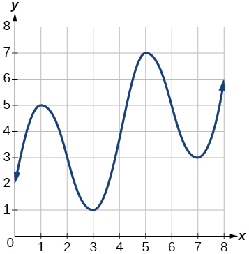
Figure 15

16. Estimate the average rate of change from \(x = 1\) to \(x = 4.\)

17. Estimate the average rate of change from \(x = 2\) to \(x = 5.\)

Solution (click to reveal)

\(\frac{4}{3}\)

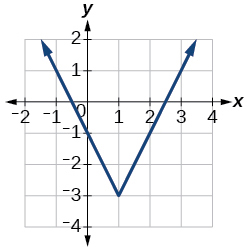
For the following exercises, use the graph of each function to estimate the intervals on which the function is increasing or decreasing.

18.

19.

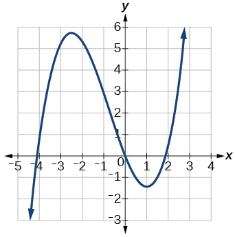
Solution (click to reveal)

increasing on \(\left( {- \infty, - 2.5} \right) \cup \left( {1,\infty} \right),\) decreasing on \(( - 2.5,\mspace{9mu} 1)\)

20.

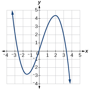
21.

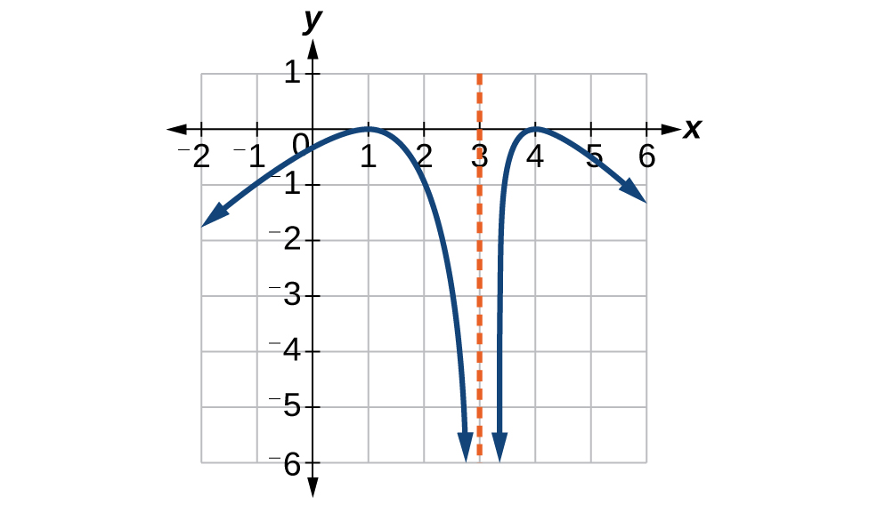
Solution (click to reveal)

increasing on \(\left( {- \infty,1} \right) \cup \left( {3,4} \right),\) decreasing on \(\left( {1,3} \right) \cup \left( {4,\infty} \right)\)

For the following exercises, consider the graph shown in Figure 16.

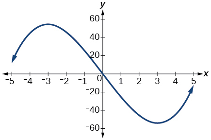
Figure 16

22. Estimate the intervals where the function is increasing or decreasing.

23. Estimate the point(s) at which the graph of \(f\) has a local maximum or a local minimum.

Solution (click to reveal)

local maximum: \(( - 3,\mspace{9mu} 60),\) local minimum: \((3,\mspace{9mu} - 60)\)

For the following exercises, consider the graph in Figure 17.

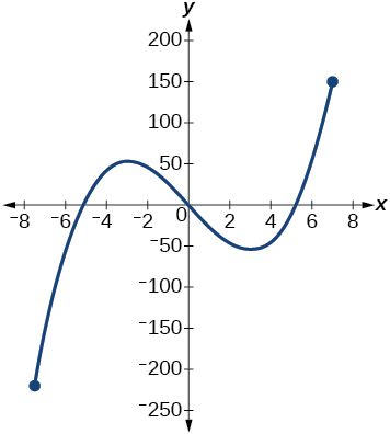
Figure 17

24. If the complete graph of the function is shown, estimate the intervals where the function is increasing or decreasing.

25. If the complete graph of the function is shown, estimate the absolute maximum and absolute minimum.

Solution (click to reveal)

absolute maximum at approximately \((7,\mspace{9mu} 150),\) absolute minimum at approximately \((-7.5,\mspace{9mu}-220)\)

Numeric

26. Table 3 gives the annual sales (in millions of dollars) of a product from 1998 to 2006. What was the average rate of change of annual sales (a) between 2001 and 2002, and (b) between 2001 and 2004?

Year	Sales (millions of dollars)
1998	201
1999	219
2000	233
2001	243
2002	249
2003	251
2004	249
2005	243
2006	233

Table 3

27. Table 4 gives the population of a town (in thousands) from 2000 to 2008. What was the average rate of change of population (a) between 2002 and 2004, and (b) between 2002 and 2006?

Year	Population (thousands)
2000	87
2001	84
2002	83
2003	80
2004	77
2005	76
2006	78
2007	81
2008	85

Table 4

Solution (click to reveal)

ⓐ \(-3000\) ⓑ \(-1250\)

For the following exercises, find the average rate of change of each function on the interval specified.

28. \(f(x) = x^{2}\) on \(\lbrack 1,\mspace{9mu} 5\rbrack\)

29. \(h(x) = 5 - 2x^{2}\) on \(\lbrack-2,\text{4}\rbrack\)

Solution (click to reveal)

-4

30. \(q(x) = x^{3}\) on \(\lbrack-4,\text{2}\rbrack\)

31. \(g(x) = 3x^{3} - 1\) on \(\lbrack-3,\text{3}\rbrack\)

Solution (click to reveal)

27

32. \(y = \frac{1}{x}\) on \(\lbrack 1,\mspace{9mu}\text{3}\rbrack\)

33. \(p(t) = \frac{\left( {t^{2} - 4} \right)\left( {t + 1} \right)}{t^{2} + 3}\) on \(\lbrack-3,\text{1}\rbrack\)

Solution (click to reveal)

–0.167

34. \(k(t) = 6t^{2} + \frac{4}{t^{3}}\) on \(\lbrack-1,3\rbrack\)

Technology

For the following exercises, use a graphing utility to estimate the local extrema of each function and to estimate the intervals on which the function is increasing and decreasing.

35. \(f(x) = x^{4} - 4x^{3} + 5\)

Solution (click to reveal)

Local minimum at \((3, - 22),\) decreasing on \(( - \infty,\mspace{9mu} 3),\) increasing on \((3,\mspace{9mu}\infty)\)

36. \(h(x) = x^{5} + 5x^{4} + 10x^{3} + 10x^{2} - 1\)

37. \(g(t) = t\sqrt{t + 3}\)

Solution (click to reveal)

Local minimum at \(( - 2, - 2),\) decreasing on \(( - 3, - 2),\) increasing on \(( - 2,\mspace{9mu}\infty)\)

38. \(k(t) = 3t^{\frac{2}{3}} - t\)

39. \(m(x) = x^{4} + 2x^{3} - 12x^{2} - 10x + 4\)

Solution (click to reveal)

Local maximum at \(( - 0.39,\mspace{9mu} 5.98),\) local minima at \(( - 3.15, - 47.62)\) and \((2.04, - 32.04),\) decreasing on \(( - \infty, - 3.15) \cup ( - 0.39,\mspace{9mu} 2.04),\) increasing on \(( - 3.15,\mspace{9mu} - 0.39) \cup (2.04,\mspace{9mu}\infty)\)

40. \(n(x) = x^{4} - 8x^{3} + 18x^{2} - 6x + 2\)

Extension

41. The graph of the function \(f\) is shown in Figure 18.

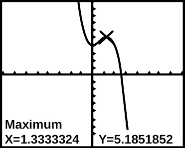
Figure 18

Based on the calculator screen shot, the point \((1.333,\mspace{9mu} 5.185)\) is which of the following?

ⓐ a relative (local) maximum of the function

ⓑ the vertex of the function

ⓒ the absolute maximum of the function

ⓓ a zero of the function

Solution (click to reveal)

A

42. Let \(f(x) = \frac{1}{x}.\) Find a number \(c\) such that the average rate of change of the function \(f\) on the interval \((1,c)\) is \(- \frac{1}{4}.\)

43. Let \(f(x) = \frac{1}{x}\) . Find the number \(b\) such that the average rate of change of \(f\) on the interval \((2,b)\) is \(- \frac{1}{10}.\)

Solution (click to reveal)

\(b = 5\)

Real-World Applications

44. At the start of a trip, the odometer on a car read 21,395. At the end of the trip, 13.5 hours later, the odometer read 22,125. Assume the scale on the odometer is in miles. What is the average speed the car traveled during this trip?

45. A driver of a car stopped at a gas station to fill up their gas tank. They looked at their watch, and the time read exactly 3:40 p.m. At this time, they started pumping gas into the tank. At exactly 3:44, the tank was full and the driver noticed that they had pumped 10.7 gallons. What is the average rate of flow of the gasoline into the gas tank?

Solution (click to reveal)

2.7 gallons per minute

46. Near the surface of the moon, the distance that an object falls is a function of time. It is given by \(d(t) = 2.6667t^{2},\) where \(t\) is in seconds and \(d(t)\) is in feet. If an object is dropped from a certain height, find the average velocity of the object from \(t = 1\) to \(t = 2.\)

47. The graph in Figure 19 illustrates the decay of a radioactive substance over \(t\) days.

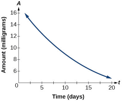
Figure 19

Use the graph to estimate the average decay rate from \(t = 5\) to \(t = 15.\)

Solution (click to reveal)

approximately –0.6 milligrams per day