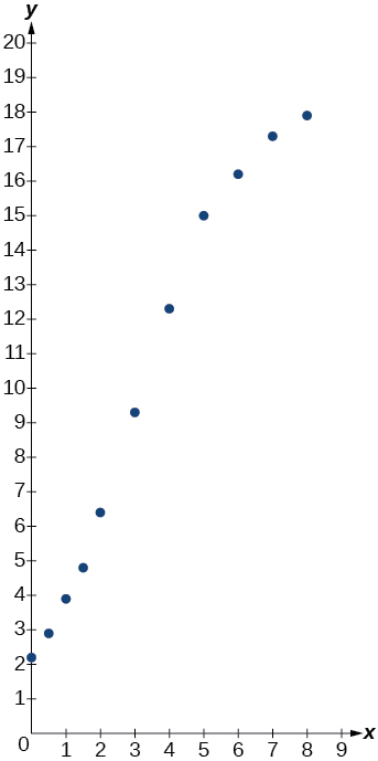
Chapter Review

Key Terms

annual percentage rate (APR) — the yearly interest rate earned by an investment account, also called nominal rate

carrying capacity — in a logistic model, the limiting value of the output

change-of-base formula — a formula for converting a logarithm with any base to a quotient of logarithms with any other base.

common logarithm — the exponent to which 10 must be raised to get \(x;\) \(\log_{10}(x)\) is written simply as \(\log(x).\)

compound interest — interest earned on the total balance, not just the principal

doubling time — the time it takes for a quantity to double

exponential growth — a model that grows by a rate proportional to the amount present

extraneous solution — a solution introduced while solving an equation that does not satisfy the conditions of the original equation

half-life — the length of time it takes for a substance to exponentially decay to half of its original quantity

logarithm — the exponent to which \(b\) must be raised to get \(x;\) written \(y = \log_{b}(x)\)

logistic growth model — a function of the form \(f(x) = \frac{c}{1 + ae^{- bx}}\) where \(\frac{c}{1 + a}\) is the initial value, \(c\) is the carrying capacity, or limiting value, and \(b\) is a constant determined by the rate of growth

natural logarithm — the exponent to which the number \(e\) must be raised to get \(x;\) \(\log_{e}(x)\) is written as \(\ln(x).\)

Newton’s Law of Cooling — the scientific formula for temperature as a function of time as an object’s temperature is equalized with the ambient temperature

nominal rate — the yearly interest rate earned by an investment account, also called annual percentage rate

order of magnitude — the power of ten, when a number is expressed in scientific notation, with one non-zero digit to the left of the decimal

power rule for logarithms — a rule of logarithms that states that the log of a power is equal to the product of the exponent and the log of its base

product rule for logarithms — a rule of logarithms that states that the log of a product is equal to a sum of logarithms

quotient rule for logarithms — a rule of logarithms that states that the log of a quotient is equal to a difference of logarithms

Key Equations

definition of the exponential function	\(f(x) = b^{x}\text{,~~where~~}b > 0,~b \neq 1\)
definition of exponential growth	\(f(x) = ab^{x},\mspace{9mu}\text{where~}a > 0,\operatorname{}b > 0,\operatorname{}b \neq 1\)
compound interest formula	\(\begin{array}{l} {A(t) = P\left( {1 + \frac{r}{n}} \right)^{nt}~,\mspace{9mu}\text{where}} \\ {A(t)\mspace{9mu}\text{is~the~account~value~at~time~}t} \\ {t\mspace{9mu}\text{is~the~number~of~years}} \\ {P\mspace{9mu}\text{is~the~initial~investment,~often~called~the~principal}} \\ {r\mspace{9mu}\text{is~the~annual~percentage~rate~(APR),~or~nominal~rate}} \\ {n\mspace{9mu}\text{is~the~number~of~compounding~periods~in~one~year}} \end{array}\)
continuous growth formula	\(A(t) = ae^{rt},\mspace{9mu}\text{where}\) \(t\) is the number of unit time periods of growth \(a\) is the starting amount (in the continuous compounding formula a is replaced with P, the principal) \(e\) is the mathematical constant, \(e \approx 2.718282\)

General Form for the Translation of the Parent Function \(f(x) = b^{x}\)

\(f(x) = ab^{x + c} + d\)

Definition of the logarithmic function	For \(~x > 0,b > 0,b \neq 1,\) \(y = \log_{b}(x)\) if and only if \(b^{y} = x.\)
Definition of the common logarithm	For \(x > 0,\) \(y = \log(x)\) if and only if \(10^{y} = x.\)
Definition of the natural logarithm	For \(x > 0,\) \(y = \ln(x)\) if and only if \(e^{y} = x.\)

General Form for the Translation of the Parent Logarithmic Function \(f(x) = \log_{b}(x)\)

\(~f(x) = a\log_{b}\left( {x + c} \right) + d\)

The Product Rule for Logarithms	\(\log_{b}(MN) = \log_{b}(M) + \log_{b}(N)\)
The Quotient Rule for Logarithms	\(\log_{b}\left( \frac{M}{N} \right) = \log_{b}M - \log_{b}N\)
The Power Rule for Logarithms	\(\log_{b}\left( M^{n} \right) = n\log_{b}M\)
The Change-of-Base Formula	\(\log_{b}M\text{=}\frac{\log_{n}M}{\log_{n}b}\mspace{9mu}\text{~~~~~~~~}n > 0,n \neq 1,b \neq 1\)

One-to-one property for exponential functions	For any algebraic expressions \(S\) and \(T\) and any positive real number \(b,\) where \(b^{S} = b^{T}\) if and only if \(S = T.\)
Definition of a logarithm	For any algebraic expression \(S\) and positive real numbers \(b~\) and \(c,\) where \(b \neq 1,\) \(\log_{b}(S) = c\) if and only if \(b^{c} = S.\)
One-to-one property for logarithmic functions	For any algebraic expressions \(S\) and \(T\) and any positive real number \(b,\) where \(b \neq 1,\) \(\log_{b}S = \log_{b}T\) if and only if \(S = T.\)

Half-life formula	If \(A = A_{0}e^{kt},\) \(k < 0,\) the half-life is \(t = - \frac{\ln(2)}{k}.\)
Carbon-14 dating	\(t = \frac{\ln\left( \frac{A}{A_{0}} \right)}{- 0.000121}.\) \(A_{0}\) is the amount of carbon-14 when the plant or animal died \(A\) is the amount of carbon-14 remaining today \(t\) is the age of the fossil in years
Doubling time formula	If \(A = A_{0}e^{kt},\) \(k > 0,\) the doubling time is \(t = \frac{\ln 2}{k}\)
Newton’s Law of Cooling	\(T(t) = Ae^{kt} + T_{s},\) where \(T_{s}\) is the ambient temperature, \(A = T(0) - T_{s},\) and \(k\) is the continuous rate of cooling.

Key Concepts

6.1 Exponential Functions

• An exponential function is defined as a function with a positive constant other than \(1\) raised to a variable exponent. See Example 1.
• A function is evaluated by solving at a specific value. See Example 2 and Example 3.
• An exponential model can be found when the growth rate and initial value are known. See Example 4.
• An exponential model can be found when the two data points from the model are known. See Example 5.
• An exponential model can be found using two data points from the graph of the model. See Example 6.
• An exponential model can be found using two data points from the graph and a calculator. See Example 7.
• The value of an account at any time \(t\) can be calculated using the compound interest formula when the principal, annual interest rate, and compounding periods are known. See Example 8.
• The initial investment of an account can be found using the compound interest formula when the value of the account, annual interest rate, compounding periods, and life span of the account are known. See Example 9.
• The number \(e\) is a mathematical constant often used as the base of real world exponential growth and decay models. Its decimal approximation is \(e \approx 2.718282.\)
• Scientific and graphing calculators have the key \(\left\lbrack e^{x} \right\rbrack\) or \(\left\lbrack {\exp(x)} \right\rbrack\) for calculating powers of \(e.\) See Example 10.
• Continuous growth or decay models are exponential models that use \(e\) as the base. Continuous growth and decay models can be found when the initial value and growth or decay rate are known. See Example 11 and Example 12.

6.2 Graphs of Exponential Functions

• The graph of the function \(f(x) = b^{x}\) has a \(y\)-intercept at \(\left( {0,~1} \right),\) domain \(\left( {- \infty,~\infty} \right),\) range \(\left( {0,~\infty} \right),\) and horizontal asymptote \(y = 0.\) See Example 1.
• If \(b > 1,\) the function is increasing. The left tail of the graph will approach the asymptote \(y = 0,\) and the right tail will increase without bound.
• If \(0 < b < 1,\) the function is decreasing. The left tail of the graph will increase without bound, and the right tail will approach the asymptote \(y = 0.\)
• The equation \(f(x) = b^{x} + d\) represents a vertical shift of the parent function \(f(x) = b^{x}.\)
• The equation \(f(x) = b^{x + c}\) represents a horizontal shift of the parent function \(f(x) = b^{x}.\) See Example 2.
• Approximate solutions of the equation \(f(x) = b^{x + c} + d\) can be found using a graphing calculator. See Example 3.
• The equation \(f(x) = ab^{x},\) where \(a > 0,\) represents a vertical stretch if \(|a| > 1\) or compression if \(0 < |a| < 1\) of the parent function \(f(x) = b^{x}.\) See Example 4.
• When the parent function \(f(x) = b^{x}\) is multiplied by \(- 1,\) the result, \(f(x) = - b^{x},\) is a reflection about the \(x\)-axis. When the input is multiplied by \(- 1,\) the result, \(f(x) = b^{- x},\) is a reflection about the \(y\)-axis. See Example 5.
• All translations of the exponential function can be summarized by the general equation \(f(x) = ab^{x + c} + d.\) See Table 3.
• Using the general equation \(f(x) = ab^{x + c} + d,\) we can write the equation of a function given its description. See Example 6.

6.3 Logarithmic Functions

• The inverse of an exponential function is a logarithmic function, and the inverse of a logarithmic function is an exponential function.
• Logarithmic equations can be written in an equivalent exponential form, using the definition of a logarithm. See Example 1.
• Exponential equations can be written in their equivalent logarithmic form using the definition of a logarithm See Example 2.
• Logarithmic functions with base \(b\) can be evaluated mentally using previous knowledge of powers of \(b.\) See Example 3 and Example 4.
• Common logarithms can be evaluated mentally using previous knowledge of powers of \(10.\) See Example 5.
• When common logarithms cannot be evaluated mentally, a calculator can be used. See Example 6.
• Real-world exponential problems with base \(10\) can be rewritten as a common logarithm and then evaluated using a calculator. See Example 7.
• Natural logarithms can be evaluated using a calculator Example 8.

6.4 Graphs of Logarithmic Functions

• To find the domain of a logarithmic function, set up an inequality showing the argument greater than zero, and solve for \(x.\) See Example 1 and Example 2

• The graph of the parent function \(f(x) = \log_{b}(x)\) has an \(x\)-intercept at \(\left( {1,0} \right),\) domain \(\left( {0,\infty} \right),\) range \(\left( {- \infty,\infty} \right),\) vertical asymptote \(x = 0,\) and
  

• if \(b > 1,\) the function is increasing.
  

• if \(0 < b < 1,\) the function is decreasing.

  See Example 3.

• The equation \(f(x) = \log_{b}\left( {x + c} \right)\) shifts the parent function \(y = \log_{b}(x)\) horizontally
  

• left \(c\) units if \(c > 0.\)
  

• right \(c\) units if \(c < 0.\)

See Example 4.

• The equation \(f(x) = \log_{b}(x) + d\) shifts the parent function \(y = \log_{b}(x)\) vertically
  
• up \(d\) units if \(d > 0.\)
  
• down \(d\) units if \(d < 0.\)

See Example 5.

• For any constant \(a > 0,\) the equation \(f(x) = a\log_{b}(x)\)
  
• stretches the parent function \(y = \log_{b}(x)\) vertically by a factor of \(a\) if \(\left| a \middle| > 1. \right.\)
  
• compresses the parent function \(y = \log_{b}(x)\) vertically by a factor of \(a\) if \(\left| a \middle| < 1. \right.\)

See Example 6 and Example 7.

• When the parent function \(y = \log_{b}(x)\) is multiplied by \(- 1,\) the result is a reflection about the \(x\)-axis. When the input is multiplied by \(- 1,\) the result is a reflection about the \(y\)-axis.
  
• The equation \(f(x) = - \log_{b}(x)\) represents a reflection of the parent function about the \(x\)-axis.
  
• The equation \(f(x) = \log_{b}\left( {- x} \right)\) represents a reflection of the parent function about the \(y\)-axis.

See Example 8.
- A graphing calculator may be used to approximate solutions to some logarithmic equations See Example 9.

• All translations of the logarithmic function can be summarized by the general equation \(~f(x) = a\log_{b}\left( {x + c} \right) + d.\) See Table 4.

• Given an equation with the general form \(f(x) = a\log_{b}\left( {x + c} \right) + d,\) we can identify the vertical asymptote \(x = - c\) for the transformation. See Example 10.

• Using the general equation \(f(x) = a\log_{b}\left( {x + c} \right) + d,\) we can write the equation of a logarithmic function given its graph. See Example 11.

6.5 Logarithmic Properties

• We can use the product rule of logarithms to rewrite the log of a product as a sum of logarithms. See Example 1.
• We can use the quotient rule of logarithms to rewrite the log of a quotient as a difference of logarithms. See Example 2.
• We can use the power rule for logarithms to rewrite the log of a power as the product of the exponent and the log of its base. See Example 3, Example 4, and Example 5.
• We can use the product rule, the quotient rule, and the power rule together to combine or expand a logarithm with a complex input. See Example 6, Example 7, and Example 8.
• The rules of logarithms can also be used to condense sums, differences, and products with the same base as a single logarithm. See Example 9, Example 10, Example 11, and Example 12.
• We can convert a logarithm with any base to a quotient of logarithms with any other base using the change-of-base formula. See Example 13.
• The change-of-base formula is often used to rewrite a logarithm with a base other than 10 and \(e\) as the quotient of natural or common logs. That way a calculator can be used to evaluate. See Example 14.

6.6 Exponential and Logarithmic Equations

• We can solve many exponential equations by using the rules of exponents to rewrite each side as a power with the same base. Then we use the fact that exponential functions are one-to-one to set the exponents equal to one another and solve for the unknown.
• When we are given an exponential equation where the bases are explicitly shown as being equal, set the exponents equal to one another and solve for the unknown. See Example 1.
• When we are given an exponential equation where the bases are not explicitly shown as being equal, rewrite each side of the equation as powers of the same base, then set the exponents equal to one another and solve for the unknown. See Example 2, Example 3, and Example 4.
• When an exponential equation cannot be rewritten with a common base, solve by taking the logarithm of each side. See Example 5.
• We can solve exponential equations with base \(e,\) by applying the natural logarithm of both sides because exponential and logarithmic functions are inverses of each other. See Example 6 and Example 7.
• After solving an exponential equation, check each solution in the original equation to find and eliminate any extraneous solutions. See Example 8.
• When given an equation of the form \(\log_{b}(S) = c,\) where \(S\) is an algebraic expression, we can use the definition of a logarithm to rewrite the equation as the equivalent exponential equation \(b^{c} = S,\) and solve for the unknown. See Example 9 and Example 10.
• We can also use graphing to solve equations with the form \(\log_{b}(S) = c.\) We graph both equations \(y = \log_{b}(S)\) and \(y = c\) on the same coordinate plane and identify the solution as the \(x\)-value of the intersecting point. See Example 11.
• When given an equation of the form \(\log_{b}S = \log_{b}T,\) where \(S\) and \(T\) are algebraic expressions, we can use the one-to-one property of logarithms to solve the equation \(S = T\) for the unknown. See Example 12.
• Combining the skills learned in this and previous sections, we can solve equations that model real world situations, whether the unknown is in an exponent or in the argument of a logarithm. See Example 13.

6.7 Exponential and Logarithmic Models

• The basic exponential function is \(f(x) = ab^{x}.\) If \(b > 1,\) we have exponential growth; if \(0 < b < 1,\) we have exponential decay.
• We can also write this formula in terms of continuous growth as \(A = A_{0}e^{kx},\) where \(A_{0}\) is the starting value. If \(A_{0}\) is positive, then we have exponential growth when \(k > 0\) and exponential decay when \(k < 0.\) See Example 1.
• In general, we solve problems involving exponential growth or decay in two steps. First, we set up a model and use the model to find the parameters. Then we use the formula with these parameters to predict growth and decay. See Example 2.
• We can find the age, \(t,\) of an organic artifact by measuring the amount, \(k,\) of carbon-14 remaining in the artifact and using the formula \(t = \frac{\ln(k)}{- 0.000121}\) to solve for \(t.\) See Example 3.
• Given a substance’s doubling time or half-time, we can find a function that represents its exponential growth or decay. See Example 4.
• We can use Newton’s Law of Cooling to find how long it will take for a cooling object to reach a desired temperature, or to find what temperature an object will be after a given time. See Example 5.
• We can use logistic growth functions to model real-world situations where the rate of growth changes over time, such as population growth, spread of disease, and spread of rumors. See Example 6.
• We can use real-world data gathered over time to observe trends. Knowledge of linear, exponential, logarithmic, and logistic graphs help us to develop models that best fit our data. See Example 7.
• Any exponential function with the form \(y = ab^{x}\) can be rewritten as an equivalent exponential function with the form \(y = A_{0}e^{kx}\) where \(k = \ln b.\) See Example 8.

6.8 Fitting Exponential Models to Data

• Exponential regression is used to model situations where growth begins slowly and then accelerates rapidly without bound, or where decay begins rapidly and then slows down to get closer and closer to zero.
• We use the command “ExpReg” on a graphing utility to fit function of the form \(y = ab^{x}\) to a set of data points. See Example 1.
• Logarithmic regression is used to model situations where growth or decay accelerates rapidly at first and then slows over time.
• We use the command “LnReg” on a graphing utility to fit a function of the form \(y = a + b\ln(x)\) to a set of data points. See Example 2.
• Logistic regression is used to model situations where growth accelerates rapidly at first and then steadily slows as the function approaches an upper limit.
• We use the command “Logistic” on a graphing utility to fit a function of the form \(y = \frac{c}{1 + ae^{- bx}}\) to a set of data points. See Example 3.

Chapter Review Exercises

Exponential Functions

1. Determine whether the function \(y = 156(0.825)^{t}\) represents exponential growth, exponential decay, or neither. Explain

Solution (click to reveal)

exponential decay; The growth factor, \(0.825,\) is between \(0\) and \(1.\)

2. The population of a herd of deer is represented by the function \(A(t) = 205{(1.13)}^{t},\) where \(t\) is given in years. To the nearest whole number, what will the herd population be after \(6\) years?

3. Find an exponential equation that passes through the points \(\text{(2,~2}\text{.25)}\) and \((5,60.75).\)

Solution (click to reveal)

\(y = 0.25(3)^{x}\)

4. Determine whether Table 13 could represent a function that is linear, exponential, or neither. If it appears to be exponential, find a function that passes through the points.

\(x\)	1	2	3	4
f(x)	3	0.9	0.27	0.081

Table 13

5. A retirement account is opened with an initial deposit of $8{,}500 and earns \(8.12\%\) interest compounded monthly. What will the account be worth in \(20\) years?

Solution (click to reveal)

\(\$ 42,888.18\)

6. Hsu-Mei wants to save $5{,}000 for a down payment on a car. To the nearest dollar, how much will she need to invest in an account now with \(7.5\%\) APR, compounded daily, in order to reach her goal in \(3\) years?

7. Does the equation \(y = 2.294e^{- 0.654t}\) represent continuous growth, continuous decay, or neither? Explain.

Solution (click to reveal)

continuous decay; the growth rate is negative.

8. Suppose an investment account is opened with an initial deposit of \(\text{\$10,500}\) earning \(6.25\%\) interest, compounded continuously. How much will the account be worth after \(25\) years?

Graphs of Exponential Functions

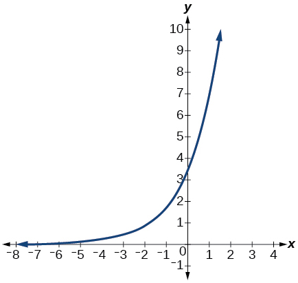
9. Graph the function \(f(x) = 3.5(2)^{x}.\) State the domain and range and give the \(y\)-intercept.

Solution (click to reveal)

domain: all real numbers; range: all real numbers strictly greater than zero; \(y\)-intercept: (0, 3.5);

10. Graph the function \(f(x) = 4\left( \frac{1}{8} \right)^{x}\) and its reflection about the \(y\)-axis on the same axes, and give the \(y\)-intercept.

11. The graph of \(f(x) = 6.5^{x}\) is reflected about the \(y\)-axis and stretched vertically by a factor of \(7.\) What is the equation of the new function, \(g(x)?\) State its \(y\)-intercept, domain, and range.

Solution (click to reveal)

\(g(x) = 7(6.5)^{- x};\) \(y\)-intercept: \((0,\mspace{9mu}\text{7});\) Domain: all real numbers; Range: all real numbers greater than \(0.\)

12. The graph below shows transformations of the graph of \(f(x) = 2^{x}.\) What is the equation for the transformation?

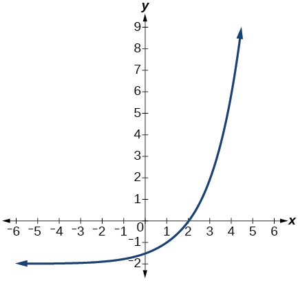
Figure 12

Logarithmic Functions

13. Rewrite \(\log_{17}(4913) = x\) as an equivalent exponential equation.

Solution (click to reveal)

\(17^{x} = 4913\)

14. Rewrite \(\ln(s) = t\) as an equivalent exponential equation.

15. Rewrite \(a^{-\frac{2}{5}} = b\) as an equivalent logarithmic equation.

Solution (click to reveal)

\(\log_{a}b = - \frac{2}{5}\)

16. Rewrite \(e^{- 3.5} = h\) as an equivalent logarithmic equation.

17. Solve for \(x\) if \(\log_{64}(x) = \frac{1}{3}\) by converting the logarithmic equation \(\log_{64}(x) = \frac{1}{3}\) to exponential form.

Solution (click to reveal)

\(x = 64^{\frac{1}{3}} = 4\)

18. Evaluate \(\log_{5}\left( \frac{1}{125} \right)\) without using a calculator.

19. Evaluate \(\log(0.000001)\) without using a calculator.

Solution (click to reveal)

\(\log\left( {\text{0}\text{.000001}} \right) = - 6\)

20. Evaluate \(\log(4.005)\) using a calculator. Round to the nearest thousandth.

21. Evaluate \(\ln\left( e^{- 0.8648} \right)\) without using a calculator.

Solution (click to reveal)

\(\ln\left( e^{- 0.8648} \right) = - 0.8648\)

22. Evaluate \(\ln\left( \sqrt[3]{18} \right)\) using a calculator. Round to the nearest thousandth.

Graphs of Logarithmic Functions

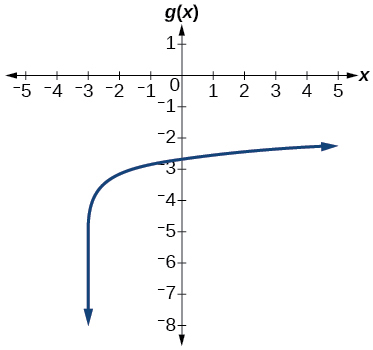
23. Graph the function \(g(x) = \log\left( {7x + 21} \right) - 4.\)

Solution (click to reveal)

24. Graph the function \(h(x) = 2\ln\left( {9 - 3x} \right) + 1.\)

25. State the domain, vertical asymptote, and end behavior of the function \(g(x) = \ln\left( {4x + 20} \right) - 17.\)

Solution (click to reveal)

Domain: \(x > - 5;\) Vertical asymptote: \(x = - 5;\) End behavior: as \(x\rightarrow - 5^{+},f(x)\rightarrow - \infty\) and as \(x\rightarrow\infty,f(x)\rightarrow\infty.\)

Logarithmic Properties

26. Rewrite \(\ln\left( {7r \cdot 11st} \right)\) in expanded form.

27. Rewrite \(\log_{8}(x) + \log_{8}(5) + \log_{8}(y) + \log_{8}(13)\) in compact form.

Solution (click to reveal)

\(\text{log}_{8}\left( {65xy} \right)\)

28. Rewrite \(\log_{m}\left( \frac{67}{83} \right)\) in expanded form.

29. Rewrite \(\ln(z) - \ln(x) - \ln(y)\) in compact form.

Solution (click to reveal)

\(\ln\left( \frac{z}{xy} \right)\)

30. Rewrite \(\ln\left( \frac{1}{x^{5}} \right)\) as a product.

31. Rewrite \(- \log_{y}\left( \frac{1}{12} \right)\) as a single logarithm.

Solution (click to reveal)

\(\text{log}_{y}(12)\)

32. Use properties of logarithms to expand \(\log\left( \frac{r^{2}s^{11}}{t^{14}} \right).\)

33. Use properties of logarithms to expand \(\ln\left( {2b\sqrt{\frac{b + 1}{b - 1}}} \right).\)

Solution (click to reveal)

\(\ln(2) + \ln(b) + \frac{\ln\left( {b + 1} \right) - \ln\left( {b - 1} \right)}{2}\)

34. Condense the expression \(5\ln(b) + \ln(c) + \frac{\ln\left( {4 - a} \right)}{2}\) to a single logarithm.

35. Condense the expression \(3\log_{7}v + 6\log_{7}w - \frac{\log_{7}u}{3}\) to a single logarithm.

Solution (click to reveal)

\(\log_{7}\left( \frac{v^{3}w^{6}}{\sqrt[3]{u}} \right)\)

36. Rewrite \(\log_{3}(12.75)\) to base \(e.\)

37. Rewrite \(5^{12x - 17} = 125\) as a logarithm. Then apply the change of base formula to solve for \(x\) using the common log. Round to the nearest thousandth.

Solution (click to reveal)

\(x = \frac{\frac{\log(125)}{\log(5)} + 17}{12} = \frac{5}{3}\)

Exponential and Logarithmic Equations

38. Solve \(216^{3x} \cdot 216^{x} = 36^{3x + 2}\) by rewriting each side with a common base.

39. Solve \(\frac{125}{\left( \frac{1}{625} \right)^{- x - 3}} = 5^{3}\) by rewriting each side with a common base.

Solution (click to reveal)

\(x = - 3\)

40. Use logarithms to find the exact solution for \(7 \cdot 17^{- 9x} - 7 = 49.\) If there is no solution, write no solution.

41. Use logarithms to find the exact solution for \(3e^{6n - 2} + 1 = - 60.\) If there is no solution, write no solution.

Solution (click to reveal)

no solution

42. Find the exact solution for \(5e^{3x} - 4 = 6\) . If there is no solution, write no solution.

43. Find the exact solution for \(2e^{5x - 2} - 9 = - 56.\) If there is no solution, write no solution.

Solution (click to reveal)

no solution

44. Find the exact solution for \(5^{2x - 3} = 7^{x + 1}.\) If there is no solution, write no solution.

45. Find the exact solution for \(e^{2x} - e^{x} - 110 = 0.\) If there is no solution, write no solution.

Solution (click to reveal)

\(x = \ln(11)\)

46. Use the definition of a logarithm to solve. \(- 5\log_{7}\left( {10n} \right) = 5.\)

47. Use the definition of a logarithm to find the exact solution for \(9 + 6\ln\left( {a + 3} \right) = 33.\)

Solution (click to reveal)

\(a = e^{4} - 3\)

48. Use the one-to-one property of logarithms to find an exact solution for \(\log_{8}(7) + \log_{8}\left( {- 4x} \right) = \log_{8}(5).\) If there is no solution, write no solution.

49. Use the one-to-one property of logarithms to find an exact solution for \(\ln(5) + \ln\left( {5x^{2} - 5} \right) = \ln(56).\) If there is no solution, write no solution.

Solution (click to reveal)

\(x = \pm \frac{9}{5}\)

50. The formula for measuring sound intensity in decibels \(D\) is defined by the equation \(D = 10\log\left( \frac{I}{I_{0}} \right),\) where \(I\) is the intensity of the sound in watts per square meter and \(I_{0} = 10^{- 12}\) is the lowest level of sound that the average person can hear. How many decibels are emitted from a large orchestra with a sound intensity of \(6.3 \cdot 10^{- 3}\) watts per square meter?

51. The population of a city is modeled by the equation \(P(t) = 256{,}114e^{0.25t}\) where \(t\) is measured in years. If the city continues to grow at this rate, how many years will it take for the population to reach one million?

Solution (click to reveal)

about \(5.45\) years

52. Find the inverse function \(f^{- 1}\) for the exponential function \(f(x) = 2 \cdot e^{x + 1} - 5.\)

53. Find the inverse function \(f^{- 1}\) for the logarithmic function \(f(x) = 0.25 \cdot \log_{2}\left( {x^{3} + 1} \right).\)

Solution (click to reveal)

\(f^{- 1}(x) = \sqrt[3]{2^{4x} - 1}\)

Exponential and Logarithmic Models

For the following exercises, use this scenario: A doctor prescribes \(300\) milligrams of a therapeutic drug that decays by about \(17\%\) each hour.

54. To the nearest minute, what is the half-life of the drug?

55. Write an exponential model representing the amount of the drug remaining in the patient’s system after \(t\) hours. Then use the formula to find the amount of the drug that would remain in the patient’s system after \(24\) hours. Round to the nearest hundredth of a gram.

Solution (click to reveal)

\(f(t) = 300(0.83)^{t};\)
\(f(24) \approx 3.43\mspace{2mu}\mspace{2mu} g\)

For the following exercises, use this scenario: A soup with an internal temperature of \(\text{350°}\) Fahrenheit was taken off the stove to cool in a \(\text{71°F}\) room. After fifteen minutes, the internal temperature of the soup was \(\text{175°F}\text{.}\)

56. Use Newton’s Law of Cooling to write a formula that models this situation.

57. How many minutes will it take the soup to cool to \(\text{85°F?}\)

Solution (click to reveal)

about \(45\) minutes

For the following exercises, use this scenario: The equation \(N(t) = \frac{1200}{1 + 199e^{- 0.625t}}\) models the number of people in a school who have heard a rumor after \(t\) days.

58. How many people started the rumor?

59. To the nearest tenth, how many days will it be before the rumor spreads to half the carrying capacity?

Solution (click to reveal)

about \(8.5\) days

60. What is the carrying capacity?

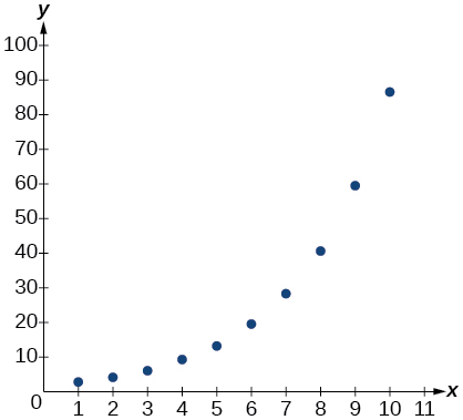
For the following exercises, enter the data from each table into a graphing calculator and graph the resulting scatter plots. Determine whether the data from the table would likely represent a function that is linear, exponential, or logarithmic.

61.

\(x\)	f(x)
1	3.05
2	4.42
3	6.4
4	9.28
5	13.46
6	19.52
7	28.3
8	41.04
9	59.5
10	86.28

Solution (click to reveal)

exponential

62.

\(x\)	f(x)
0.5	18.05
1	17
3	15.33
5	14.55
7	14.04
10	13.5
12	13.22
13	13.1
15	12.88
17	12.69
20	12.45

63. Find a formula for an exponential equation that goes through the points \(\left( {- 2{,}100} \right)\) and \(\left( {0,4} \right).\) Then express the formula as an equivalent equation with base \(e\).

Solution (click to reveal)

\(y = 4(0.2)^{x};\) \(y = 4e^{\text{-1.609438}x}\)

Fitting Exponential Models to Data

64. What is the carrying capacity for a population modeled by the logistic equation \(P(t) = \frac{250{,}000}{1 + 499e^{- 0.45t}}?\) What is the initial population for the model?

65. The population of a culture of bacteria is modeled by the logistic equation \(\mspace{9mu} P(t) = \frac{14{,}250}{1 + 29e^{- 0.62t}},\) where \(t\) is in days. To the nearest tenth, how many days will it take the culture to reach \(75\%\) of its carrying capacity?

Solution (click to reveal)

about \(7.2\) days

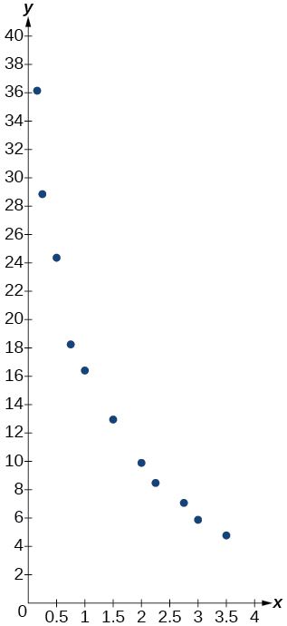
For the following exercises, use a graphing utility to create a scatter diagram of the data given in the table. Observe the shape of the scatter diagram to determine whether the data is best described by an exponential, logarithmic, or logistic model. Then use the appropriate regression feature to find an equation that models the data. When necessary, round values to five decimal places.

66.

\(x\)	f(x)
1	409.4
2	260.7
3	170.4
4	110.6
5	74
6	44.7
7	32.4
8	19.5
9	12.7
10	8.1

67.

\(x\)	f(x)
0.15	36.21
0.25	28.88
0.5	24.39
0.75	18.28
1	16.5
1.5	12.99
2	9.91
2.25	8.57
2.75	7.23
3	5.99
3.5	4.81

Solution (click to reveal)

logarithmic; \(y = 16.68718 - 9.71860\ln(x)\)

68.

\(x\)	f(x)
0	9
2	22.6
4	44.2
5	62.1
7	96.9
8	113.4
10	133.4
11	137.6
15	148.4
17	149.3

Practice Test

1. The population of a pod of bottlenose dolphins is modeled by the function \(A(t) = 8{(1.17)}^{t},\) where \(t\) is given in years. To the nearest whole number, what will the pod population be after \(3\) years?

Solution (click to reveal)

About 13 dolphins.

2. Find an exponential equation that passes through the points \(\text{(0, 4)}\) and \(\text{(2, 9)}\text{.}\)

3. Drew wants to save $2{,}500 to go to the next World Cup. To the nearest dollar, how much will he need to invest in an account now with \(6.25\%\) APR, compounding daily, in order to reach his goal in \(4\) years?

Solution (click to reveal)

\(\$ 1,947\)

4. An investment account was opened with an initial deposit of $9{,}600 and earns \(7.4\%\) interest, compounded continuously. How much will the account be worth after \(15\) years?

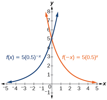
5. Graph the function \(f(x) = 5(0.5)^{- x}\) and its reflection across the \(y\)-axis on the same axes, and give the \(y\)-intercept.

Solution (click to reveal)

\(y\)-intercept: \((0,\mspace{9mu}\text{5})\)

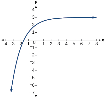
6. The graph shows transformations of the graph of \(f(x) = \left( \frac{1}{2} \right)^{x}.\) What is the equation for the transformation?

7. Rewrite \(\log_{8.5}(614.125) = a\) as an equivalent exponential equation.

Solution (click to reveal)

\(8.5^{a} = 614.125\)

8. Rewrite \(e^{\frac{1}{2}} = m\) as an equivalent logarithmic equation.

9. Solve for \(x\) by converting the logarithmic equation \(log_{\frac{1}{7}}(x) = 2\) to exponential form.

Solution (click to reveal)

\(x = \left( \frac{1}{7} \right)^{2} = \frac{1}{49}\)

10. Evaluate \(\log(10{,}000,000)\) without using a calculator.

11. Evaluate \(\ln(0.716)\) using a calculator. Round to the nearest thousandth.

Solution (click to reveal)

\(\ln(0.716) \approx - 0.334\)

12. Graph the function \(g(x) = \log\left( {12 - 6x} \right) + 3.\)

13. State the domain, vertical asymptote, and end behavior of the function \(f(x) = \log_{5}\left( {39 - 13x} \right) + 7.\)

Solution (click to reveal)

Domain: \(x < 3;\) Vertical asymptote: \(x = 3;\) End behavior: \(x\rightarrow 3^{-},f(x)\rightarrow - \infty\) and \(x\rightarrow - \infty,f(x)\rightarrow\infty\)

14. Rewrite \(\log\left( {17a \cdot 2b} \right)\) as a sum.

15. Rewrite \(\log_{t}(96) - \log_{t}(8)\) in compact form.

Solution (click to reveal)

\(\log_{t}(12)\)

16. Rewrite \(\log_{8}\left( a^{\frac{1}{b}} \right)\) as a product.

17. Use properties of logarithm to expand \(\ln\left( {y^{3}z^{2} \cdot \sqrt[3]{x - 4}} \right).\)

Solution (click to reveal)

\(3\ \ln(y) + 2\ln(z) + \frac{\ln\left( {x - 4} \right)}{3}\)

18. Condense the expression \(4\ln(c) + \ln(d) + \frac{\ln(a)}{3} + \frac{\ln\left( {b + 3} \right)}{3}\) to a single logarithm.

19. Rewrite \(16^{3x - 5} = 1000\) as a logarithm. Then apply the change of base formula to solve for \(x\) using the natural log. Round to the nearest thousandth.

Solution (click to reveal)

\(x = \frac{\frac{\ln(1000)}{\ln(16)} + 5}{3} \approx 2.497\)

20. Solve \(\left( \frac{1}{81} \right)^{x} \cdot \frac{1}{243} = \left( \frac{1}{9} \right)^{- 3x - 1}\) by rewriting each side with a common base.

21. Use logarithms to find the exact solution for \(- 9e^{10a - 8} - 5 = - 41\) . If there is no solution, write no solution.

Solution (click to reveal)

\(a = \frac{\ln(4) + 8}{10}\)

22. Find the exact solution for \(10e^{4x + 2} + 5 = 56.\) If there is no solution, write no solution.

23. Find the exact solution for \(- 5e^{- 4x - 1} - 4 = 64.\) If there is no solution, write no solution.

Solution (click to reveal)

no solution

24. Find the exact solution for \(2^{x - 3} = 6^{2x - 1}.\) If there is no solution, write no solution.

25. Find the exact solution for \(e^{2x} - e^{x} - 72 = 0.\) If there is no solution, write no solution.

Solution (click to reveal)

\(x = \ln(9)\)

26. Use the definition of a logarithm to find the exact solution for \(4\log\left( {2n} \right) - 7 = - 11\)

27. Use the one-to-one property of logarithms to find an exact solution for \(\log\left( {4x^{2} - 10} \right) + \log(3) = \log(51)\) If there is no solution, write no solution.

Solution (click to reveal)

\(x = \pm \frac{3\sqrt{3}}{2}\)

28. The formula for measuring sound intensity in decibels \(D\) is defined by the equation \(D = 10\log\left( \frac{I}{I_{0}} \right),\) where \(I\) is the intensity of the sound in watts per square meter and \(I_{0} = 10^{- 12}\) is the lowest level of sound that the average person can hear. How many decibels are emitted from a rock concert with a sound intensity of \(4.7 \cdot 10^{- 1}\) watts per square meter?

29. A radiation safety officer is working with \(112\) grams of a radioactive substance. After \(17\) days, the sample has decayed to \(80\) grams. Rounding to five significant digits, write an exponential equation representing this situation. To the nearest day, what is the half-life of this substance?

Solution (click to reveal)

\(f(t) = 112e^{- .019792t};\) half-life: about \(35\) days

30. Write the formula found in the previous exercise as an equivalent equation with base \(e.\) Express the exponent to five significant digits.

31. A bottle of soda with a temperature of \(\text{71°}\) Fahrenheit was taken off a shelf and placed in a refrigerator with an internal temperature of \(\text{35° F}\text{.}\) After ten minutes, the internal temperature of the soda was \(\text{63° F}\text{.}\) Use Newton’s Law of Cooling to write a formula that models this situation. To the nearest degree, what will the temperature of the soda be after one hour?

Solution (click to reveal)

\(T(t) = 36e^{- 0.025131t} + 35;T(60) \approx 43^{\text{o}}\text{F}\)

32. The population of a wildlife habitat is modeled by the equation \(P(t) = \frac{360}{1 + 6.2e^{- 0.35t}},\) where \(t\) is given in years. How many animals were originally transported to the habitat? How many years will it take before the habitat reaches half its capacity?

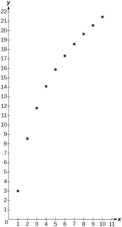
33. Enter the data from into a graphing calculator and graph the resulting scatter plot. Determine whether the data from the table would likely represent a function that is linear, exponential, or logarithmic.

\(x\)	f(x)
1	3
2	8.55
3	11.79
4	14.09
5	15.88
6	17.33
7	18.57
8	19.64
9	20.58
10	21.42

Solution (click to reveal)

logarithmic

34. The population of a lake of fish is modeled by the logistic equation \(P(t) = \frac{16{,}120}{1 + 25e^{- 0.75t}},\) where \(t\) is time in years. To the nearest hundredth, how many years will it take the lake to reach \(80\%\) of its carrying capacity?

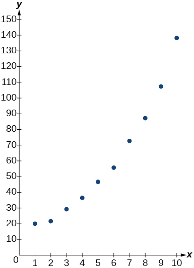
For the following exercises, use a graphing utility to create a scatter diagram of the data given in the table. Observe the shape of the scatter diagram to determine whether the data is best described by an exponential, logarithmic, or logistic model. Then use the appropriate regression feature to find an equation that models the data. When necessary, round values to five decimal places.

35.

\(x\)	f(x)
1	20
2	21.6
3	29.2
4	36.4
5	46.6
6	55.7
7	72.6
8	87.1
9	107.2
10	138.1

Solution (click to reveal)

exponential; \(y = 15.10062(1.24621)^{x}\)

36.

\(x\)	f(x)
3	13.98
4	17.84
5	20.01
6	22.7
7	24.1
8	26.15
9	27.37
10	28.38
11	29.97
12	31.07
13	31.43

37.

\(x\)	f(x)
0	2.2
0.5	2.9
1	3.9
1.5	4.8
2	6.4
3	9.3
4	12.3
5	15
6	16.2
7	17.3
8	17.9

Solution (click to reveal)

logistic; \(y = \frac{18.41659}{1 + 7.54644e^{- 0.68375x}}\)