3.5 Transformation of Functions
Figure 1 (credit: “Misko”/Flickr)
We all know that a flat mirror enables us to see an accurate image of ourselves and whatever is behind us. When we tilt the mirror, the images we see may shift horizontally or vertically. But what happens when we bend a flexible mirror? Like a carnival funhouse mirror, it presents us with a distorted image of ourselves, stretched or compressed horizontally or vertically. In a similar way, we can distort or transform mathematical functions to better adapt them to describing objects or processes in the real world. In this section, we will take a look at several kinds of transformations.
3.5.1 Graphing Functions Using Vertical and Horizontal Shifts
Often when given a problem, we try to model the scenario using mathematics in the form of words, tables, graphs, and equations. One method we can employ is to adapt the basic graphs of the toolkit functions to build new models for a given scenario. There are systematic ways to alter functions to construct appropriate models for the problems we are trying to solve.
Identifying Vertical Shifts
One simple kind of transformation involves shifting the entire graph of a function up, down, right, or left. The simplest shift is a vertical shift, moving the graph up or down, because this transformation involves adding a positive or negative constant to the function. In other words, we add the same constant to the output value of the function regardless of the input. For a function \(g(x) = f(x) + k,\) the function \(f(x)\) is shifted vertically \(k\) units. See Figure 2 for an example.
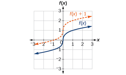
Figure 2 Vertical shift by \(k = 1\) of the cube root function \(f(x) = \sqrt[3]{x}.\)
To help you visualize the concept of a vertical shift, consider that \(y = f(x).\) Therefore, \(f(x) + k\) is equivalent to \(y + k.\) Every unit of \(y\) is replaced by \(y + k,\) so the \(y\)-value increases or decreases depending on the value of \(k.\) The result is a shift upward or downward.
To regulate temperature in a green building, airflow vents near the roof open and close throughout the day. Figure 3 shows the area of open vents \(V\) (in square feet) throughout the day in hours after midnight, \(t.\) During the summer, the facilities manager decides to try to better regulate temperature by increasing the amount of open vents by 20 square feet throughout the day and night. Sketch a graph of this new function.
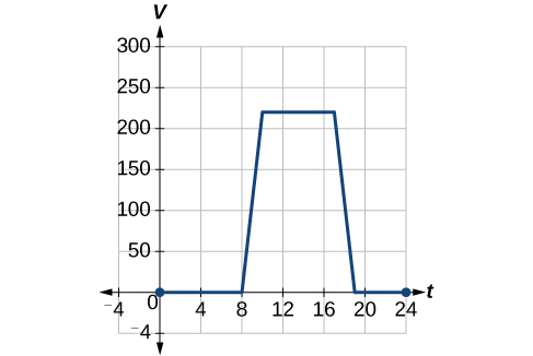
Figure 3
Solution (click to reveal)
We can sketch a graph of this new function by adding 20 to each of the output values of the original function. This will have the effect of shifting the graph vertically up, as shown in Figure 4.
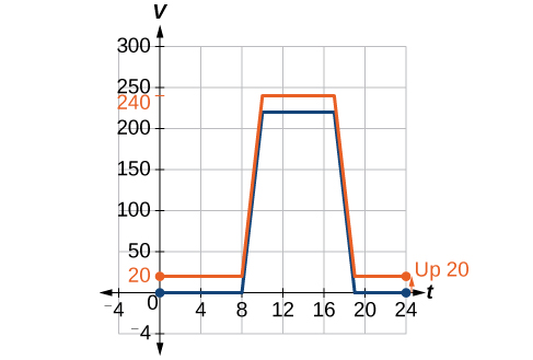
Figure 4
Notice that in Figure 4, for each input value, the output value has increased by 20, so if we call the new function \(S(t),\) we could write
\[S(t) = V(t) + 20\]
This notation tells us that, for any value of \(t,S(t)\) can be found by evaluating the function \(V\) at the same input and then adding 20 to the result. This defines \(S\) as a transformation of the function \(V,\) in this case a vertical shift up 20 units. Notice that, with a vertical shift, the input values stay the same and only the output values change. See Table 1.
| \(t\) | 0 | 8 | 10 | 17 | 19 | 24 |
| \(V(t)\) | 0 | 0 | 220 | 220 | 0 | 0 |
| \(S(t)\) | 20 | 20 | 240 | 240 | 20 | 20 |
Table 1
Identifying Horizontal Shifts
We just saw that the vertical shift is a change to the output, or outside, of the function. We will now look at how changes to input, on the inside of the function, change its graph and meaning. A shift to the input results in a movement of the graph of the function left or right in what is known as a horizontal shift, shown in Figure 5.
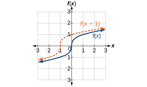
Figure 5 Horizontal shift of the function \(f(x) = \sqrt[3]{x}.\) Note that \((x + 1)\) means \(h = –1\), which shifts the graph to the left, that is, towards negative values of \(x.\)
For example, if \(f(x) = x^{2},\) then \(g(x) = {(x - 2)}^{2}\) is a new function. Each input is reduced by 2 prior to squaring the function. The result is that the graph is shifted 2 units to the right, because we would need to increase the prior input by 2 units to yield the same output value as given in \(f.\)
Returning to our building airflow example from Figure 3, suppose that in autumn the facilities manager decides that the original venting plan starts too late, and wants to begin the entire venting program 2 hours earlier. Sketch a graph of the new function.
Solution (click to reveal)
We can set \(V(t)\) to be the original program and \(F(t)\) to be the revised program.
\[\begin{array}{rcl} {V(t)} & = & \text{the~original~venting~plan} \\ {F(t)} & = & \text{starting~2~hrs~sooner} \end{array}\]
In the new graph, at each time, the airflow is the same as the original function \(V\) was 2 hours later. For example, in the original function \(V,\) the airflow starts to change at 8 a.m., whereas for the function \(F,\) the airflow starts to change at 6 a.m. The comparable function values are \(V(8) = F(6).\) See Figure 6. Notice also that the vents first opened to \(220{\mspace{9mu}\text{ft}}^{2}\) at 10 a.m. under the original plan, while under the new plan the vents reach \(220{\mspace{9mu}\text{ft}}^{\text{2}}\) at
8 a.m., so \(V(10) = F(8).\)
In both cases, we see that, because \(F(t)\) starts 2 hours sooner, \(h = - 2.\) That means that the same output values are reached when \(F(t) = V(t - \left( {- 2} \right)) = V\left( {t + 2} \right).\)
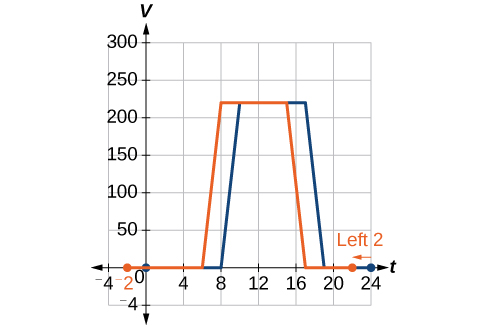
Figure 6
Note that \(V(t + 2)\) has the effect of shifting the graph to the left.
Horizontal changes or “inside changes” affect the domain of a function (the input) instead of the range and often seem counterintuitive. The new function \(F(t)\) uses the same outputs as \(V(t),\) but matches those outputs to inputs 2 hours earlier than those of \(V(t).\) Said another way, we must add 2 hours to the input of \(V\) to find the corresponding output for \(F:F(t) = V(t + 2).\)
A function \(f(x)\) is given in Table 4. Create a table for the function \(g(x) = f(x - 3).\)
| \(x\) | 2 | 4 | 6 | 8 |
| \(f(x)\) | 1 | 3 | 7 | 11 |
Table 4
Solution (click to reveal)
The formula \(g(x) = f(x - 3)\) tells us that the output values of \(g\) are the same as the output value of \(f\) when the input value is 3 less than the original value. For example, we know that \(f(2) = 1.\) To get the same output from the function \(g,\) we will need an input value that is 3 larger. We input a value that is 3 larger for \(g(x)\) because the function takes 3 away before evaluating the function \(f.\)
\[\begin{array}{ccl} {g(5)} & = & {f(5 - 3)} \\ & = & {f(2)} \\ & = & 1 \end{array}\]
We continue with the other values to create Table 5.
| \(x\) | 5 | 7 | 9 | 11 |
| \(x - 3\) | 2 | 4 | 6 | 8 |
| \(f(x–3)\) | 1 | 3 | 7 | 11 |
| \(g(x)\) | 1 | 3 | 7 | 11 |
Table 5
The result is that the function \(g(x)\) has been shifted to the right by 3. Notice the output values for \(g(x)\) remain the same as the output values for \(f(x),\) but the corresponding input values, \(x,\) have shifted to the right by 3. Specifically, 2 shifted to 5, 4 shifted to 7, 6 shifted to 9, and 8 shifted to 11.
Figure 7 represents both of the functions. We can see the horizontal shift in each point.
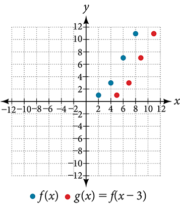
Figure 7
Figure 8 represents a transformation of the toolkit function \(f(x) = x^{2}.\) Relate this new function \(g(x)\) to \(f(x),\) and then find a formula for \(g(x).\)
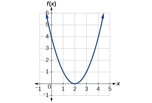
Figure 8
Solution (click to reveal)
Notice that the graph is identical in shape to the \(f(x) = x^{2}\) function, but the \(x\)-values are shifted to the right 2 units. The vertex used to be at (0,0), but now the vertex is at (2,0). The graph is the basic quadratic function shifted 2 units to the right, so
\[g(x) = f(x - 2)\]
Notice how we must input the value \(x = 2\) to get the output value \(y = 0;\) thex-values must be 2 units larger because of the shift to the right by 2 units. We can then use the definition of the \(f(x)\) function to write a formula for \(g(x)\) by evaluating \(f(x - 2).\)
\[\begin{array}{rcl} {f(x)} & = & x^{2} \\ {g(x)} & = & {f(x - 2)} \\ {g(x)} & = & {f(x - 2) = {(x - 2)}^{2}} \end{array}\]
To determine whether the shift is \(+ 2\) or \(- 2\) , consider a single reference point on the graph. For a quadratic, looking at the vertex point is convenient. In the original function, \(f(0) = 0.\) In our shifted function, \(g(2) = 0.\) To obtain the output value of 0 from the function \(f,\) we need to decide whether a plus or a minus sign will work to satisfy \(g(2) = f(x - 2) = f(0) = 0.\) For this to work, we will need to subtract 2 units from our input values.
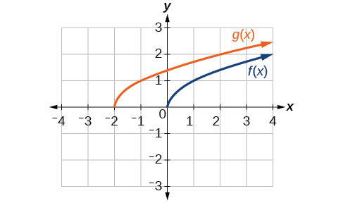
Given the function \(f(x) = \sqrt{x},\) graph the original function \(f(x)\) and the transformation \(g(x) = f(x + 2)\) on the same axes. Is this a horizontal or a vertical shift? Which way is the graph shifted and by how many units?
Solution (click to reveal)
The graphs of \(f(x)\) and \(g(x)\) are shown below. The transformation is a horizontal shift. The function is shifted to the left by 2 units.
Combining Vertical and Horizontal Shifts
Now that we have two transformations, we can combine them. Vertical shifts are outside changes that affect the output (\(y\)-) values and shift the function up or down. Horizontal shifts are inside changes that affect the input (\(x\)-) values and shift the function left or right. Combining the two types of shifts will cause the graph of a function to shift up or down and left or right.
Given \(f(x) = |x|,\) sketch a graph of \(h(x) = f(x + 1) - 3.\)
Solution (click to reveal)
The function \(f\) is our toolkit absolute value function. We know that this graph has a V shape, with the point at the origin. The graph of \(h\) has transformed \(f\) in two ways: \(f(x + 1)\) is a change on the inside of the function, giving a horizontal shift left by 1, and the subtraction by 3 in \(f(x + 1) - 3\) is a change to the outside of the function, giving a vertical shift down by 3. The transformation of the graph is illustrated in Figure 9.
Let us follow one point of the graph of \(f(x) = |x|.\)
- The point \((0,0)\) is transformed first by shifting left 1 unit: \((0,0)\rightarrow(-1,0)\)
- The point \((-1,0)\) is transformed next by shifting down 3 units: \((-1,0)\rightarrow(-1,-3)\)
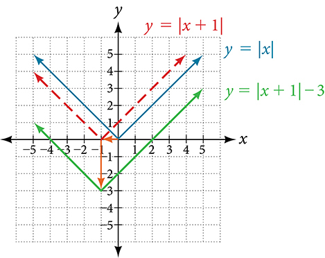
Figure 9
Figure 10 shows the graph of \(h.\)
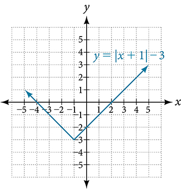
Figure 10
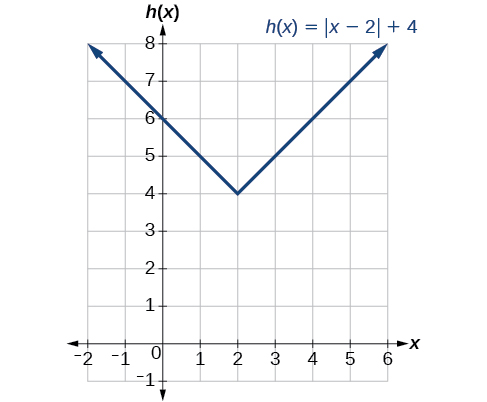
Given \(f(x) = |x|,\) sketch a graph of \(h(x) = f(x - 2) + 4.\)
Solution (click to reveal)
Write a formula for the graph shown in Figure 11, which is a transformation of the toolkit square root function.
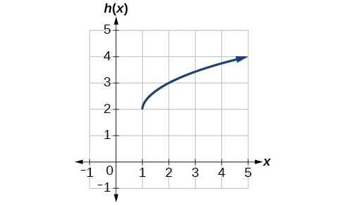
Figure 11
Solution (click to reveal)
The graph of the toolkit function starts at the origin, so this graph has been shifted 1 to the right and up 2. In function notation, we could write that as
\[h(x) = f(x - 1) + 2\]
Using the formula for the square root function, we can write
\[h(x) = \sqrt{x - 1} + 2\]
Note that this transformation has changed the domain and range of the function. This new graph has domain \(\lbrack 1,\infty)\) and range \(\lbrack 2,\infty).\)
3.5.2 Graphing Functions Using Reflections about the Axes
Another transformation that can be applied to a function is a reflection over the \(x\)- or \(y\)-axis. A vertical reflection reflects a graph vertically across the \(x\)-axis, while a horizontal reflection reflects a graph horizontally across the \(y\)-axis. The reflections are shown in Figure 12.
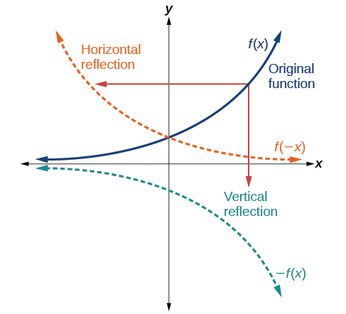
Figure 12 Vertical and horizontal reflections of a function.
Notice that the vertical reflection produces a new graph that is a mirror image of the base or original graph about the \(x\)-axis. The horizontal reflection produces a new graph that is a mirror image of the base or original graph about the \(y\)-axis.
Reflect the graph of \(s(t) = \sqrt{t}\) (a) vertically and (b) horizontally.
Solution (click to reveal)
ⓐ Reflecting the graph vertically means that each output value will be reflected over the horizontal \(t\)-axis as shown in Figure 13.
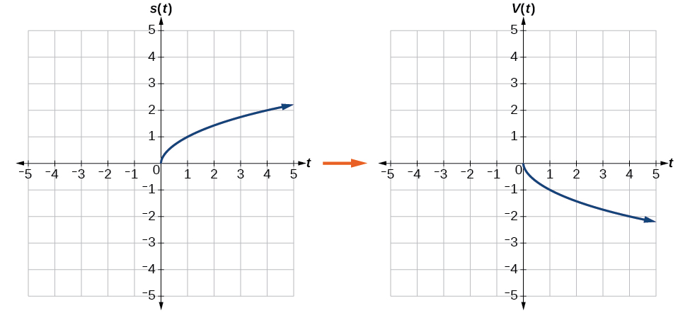
Figure 13 Vertical reflection of the square root function
Because each output value is the opposite of the original output value, we can write
\[V(t) = - s(t)\mspace{9mu}\text{or~}V(t) = - \sqrt{t}\]
Notice that this is an outside change, or vertical shift, that affects the output \(s(t)\) values, so the negative sign belongs outside of the function.
ⓑ Reflecting horizontally means that each input value will be reflected over the vertical axis as shown in Figure 14.
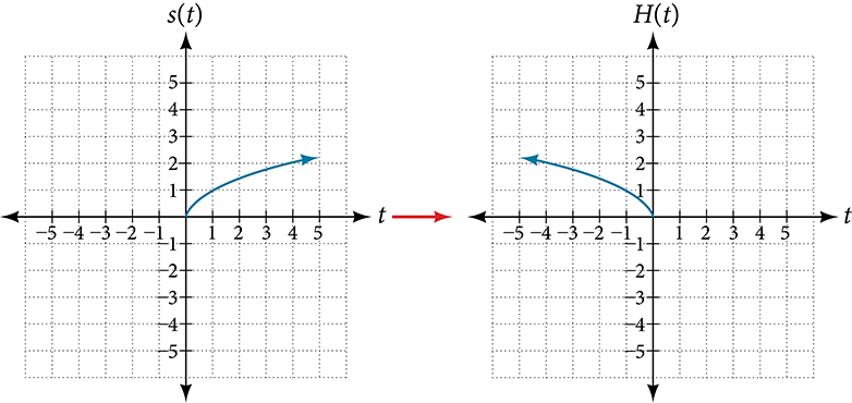
Figure 14 Horizontal reflection of the square root function
Because each input value is the opposite of the original input value, we can write
\[H(t) = s( - t)\mspace{9mu}\text{or~}H(t) = \sqrt{- t}\]
Notice that this is an inside change or horizontal change that affects the input values, so the negative sign is on the inside of the function. Note that these transformations can affect the domain and range of the functions. While the original square root function has domain \(\lbrack 0,\infty)\) and range \(\lbrack 0,\infty),\) the vertical reflection gives the \(V(t)\) function the range \(\left( {- \infty,\mspace{9mu} 0} \right\rbrack\) and the horizontal reflection gives the \(H(t)\) function the domain \(\left( {- \infty,\mspace{9mu} 0} \right\rbrack.\)
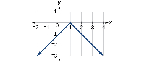
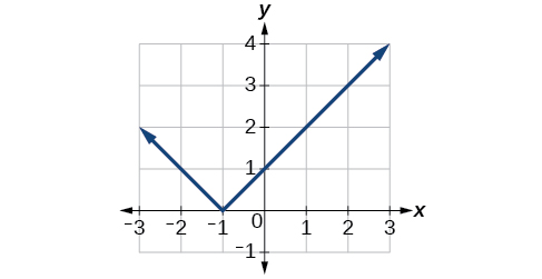
Reflect the graph of \(\left. f(x) = \middle| x - 1 \right|\) (a) vertically and (b) horizontally.
Solution (click to reveal)
ⓐ
ⓑ
A common model for learning has an equation similar to \(k(t) = - 2^{- t} + 1,\) where \(k\) is the percentage of mastery that can be achieved after \(t\) practice sessions. This is a transformation of the function \(f(t) = 2^{t}\) shown in Figure 15. Sketch a graph of \(k(t).\)
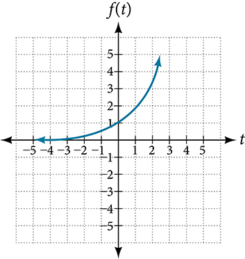
Figure 15
Solution (click to reveal)
This equation combines three transformations into one equation.
- A horizontal reflection: \(f(\text{−}t) = 2^{- t}\)
- A vertical reflection: \(- f(\text{−}t) = - 2^{- t}\)
- A vertical shift: \(- f(\text{−}t) + 1 = - 2^{- t} + 1\)
We can sketch a graph by applying these transformations one at a time to the original function. Let us follow two points through each of the three transformations. We will choose the points (0, 1) and (1, 2).
- First, we apply a horizontal reflection: (0, 1) (–1, 2).
- Then, we apply a vertical reflection: (0, -1) (-1, –2)
- Finally, we apply a vertical shift: (0, 0) (-1, -1)).
This means that the original points, (0,1) and (1,2) become (0,0) and (-1,-1) after we apply the transformations.
In Figure 16, the first graph results from a horizontal reflection. The second results from a vertical reflection. The third results from a vertical shift up 1 unit.
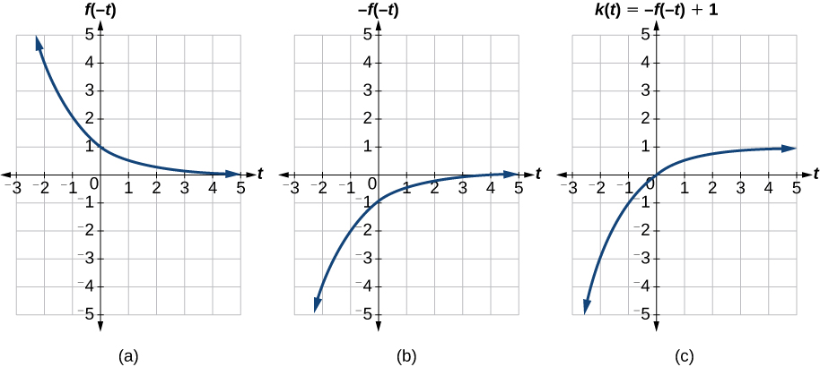
Figure 16
As a model for learning, this function would be limited to a domain of \(t \geq 0,\) with corresponding range \(\lbrack 0,1).\)
Given the toolkit function \(f(x) = x^{2},\) graph \(g(x) = - f(x)\) and \(h(x) = f( - x).\) Take note of any surprising behavior for these functions.
Solution (click to reveal)
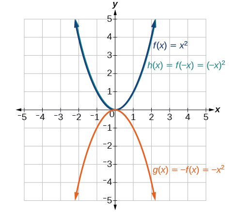
Notice: \(g(x) = f( - x)\) looks the same as \(f(x)\) .
3.5.3 Determining Even and Odd Functions
Some functions exhibit symmetry so that reflections result in the original graph. For example, horizontally reflecting the toolkit functions \(f(x) = x^{2}\) or \(f(x) = |x|\) will result in the original graph. We say that these types of graphs are symmetric about the \(y\)-axis. A function whose graph is symmetric about the \(y\)-axis is called an even function.
If the graphs of \(f(x) = x^{3}\) or \(f(x) = \frac{1}{x}\) were reflected over both axes, the result would be the original graph, as shown in Figure 17.
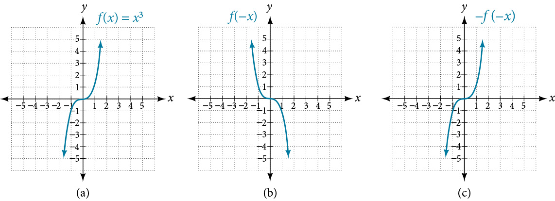
Figure 17 (a) The cubic toolkit function (b) Horizontal reflection of the cubic toolkit function (c) Horizontal and vertical reflections reproduce the original cubic function.
We say that these graphs are symmetric about the origin. A function with a graph that is symmetric about the origin is called an odd function.
Note: A function can be neither even nor odd if it does not exhibit either symmetry. For example, \(f(x) = 2^{x}\) is neither even nor odd. Also, the only function that is both even and odd is the constant function \(f(x) = 0.\)
Is the function \(f(x) = x^{3} + 2x\) even, odd, or neither?
Solution (click to reveal)
Without looking at a graph, we can determine whether the function is even or odd by finding formulas for the reflections and determining if they return us to the original function. Let’s begin with the rule for even functions.
\[f( - x) = {( - x)}^{3} + 2( - x) = - x^{3} - 2x\]
This does not return us to the original function, so this function is not even. We can now test the rule for odd functions.
\[- f( - x) = - \left( {- x^{3} - 2x} \right) = x^{3} + 2x\]
Because \(- f( - x) = f(x),\) this is an odd function.
Consider the graph of \(f\) in Figure 18. Notice that the graph is symmetric about the origin. For every point \(\left( {x,y} \right)\) on the graph, the corresponding point \(\left( {- x, - y} \right)\) is also on the graph. For example, (1, 3) is on the graph of \(f,\) and the corresponding point \((-1,-3)\) is also on the graph.
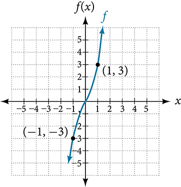
Figure 18
3.5.4 Graphing Functions Using Stretches and Compressions
Adding a constant to the inputs or outputs of a function changed the position of a graph with respect to the axes, but it did not affect the shape of a graph. We now explore the effects of multiplying the inputs or outputs by some quantity.
We can transform the inside (input values) of a function or we can transform the outside (output values) of a function. Each change has a specific effect that can be seen graphically.
Vertical Stretches and Compressions
When we multiply a function by a positive constant, we get a function whose graph is stretched or compressed vertically in relation to the graph of the original function. If the constant is greater than 1, we get a vertical stretch; if the constant is between 0 and 1, we get avertical compression. Figure 19 shows a function multiplied by constant factors 2 and 0.5 and the resulting vertical stretch and compression.
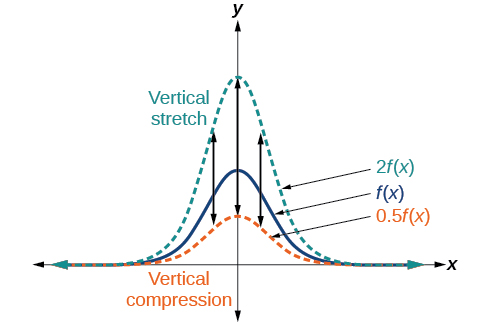
Figure 19 Vertical stretch and compression
A function \(P(t)\) models the population of fruit flies. The graph is shown in Figure 20.
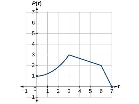
Figure 20
A scientist is comparing this population to another population, \(Q,\) whose growth follows the same pattern, but is twice as large. Sketch a graph of this population.
Solution (click to reveal)
Because the population is always twice as large, the new population’s output values are always twice the original function’s output values. Graphically, this is shown in Figure 21.
If we choose four reference points, (0, 1), (3, 3), (6, 2) and (7, 0) we will multiply all of the outputs by 2.
The following shows where the new points for the new graph will be located.
\[\begin{array}{l} {\left( {0,\mspace{9mu} 1} \right)\rightarrow\left( {0,\mspace{9mu} 2} \right)} \\ {\left( {3,\mspace{9mu} 3} \right)\rightarrow\left( {3,\mspace{9mu} 6} \right)} \\ {\left( {6,\mspace{9mu} 2} \right)\rightarrow\left( {6,\mspace{9mu} 4} \right)} \\ {\left( {7,\mspace{9mu} 0} \right)\rightarrow\left( {7,\mspace{9mu} 0} \right)} \end{array}\]
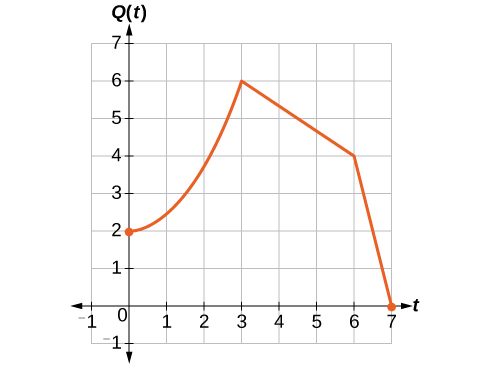
Figure 21
Symbolically, the relationship is written as
\[Q(t) = 2P(t)\]
This means that for any input \(t,\) the value of the function \(Q\) is twice the value of the function \(P.\) Notice that the effect on the graph is a vertical stretching of the graph, where every point doubles its distance from the horizontal axis. The input values, \(t,\) stay the same while the output values are twice as large as before.
The graph in Figure 22 is a transformation of the toolkit function \(f(x) = x^{3}.\) Relate this new function \(g(x)\) to \(f(x),\) and then find a formula for \(g(x).\)
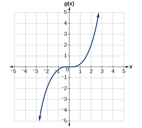
Figure 22
Solution (click to reveal)
When trying to determine a vertical stretch or shift, it is helpful to look for a point on the graph that is relatively clear. In this graph, it appears that \(g(2) = 2.\) With the basic cubic function at the same input, \(f(2) = 2^{3} = 8.\) Based on that, it appears that the outputs of \(g\) are \(\frac{1}{4}\) the outputs of the function \(f\) because \(g(2) = \frac{1}{4}f(2).\) From this we can fairly safely conclude that \(g(x) = \frac{1}{4}f(x).\)
We can write a formula for \(g\) by using the definition of the function \(f.\)
\[g(x) = \frac{1}{4}f(x) = \frac{1}{4}x^{3}\]
Horizontal Stretches and Compressions
Now we consider changes to the inside of a function. When we multiply a function’s input by a positive constant, we get a function whose graph is stretched or compressed horizontally in relation to the graph of the original function. If the constant is between 0 and 1, we get a horizontal stretch; if the constant is greater than 1, we get a horizontal compression of the function.
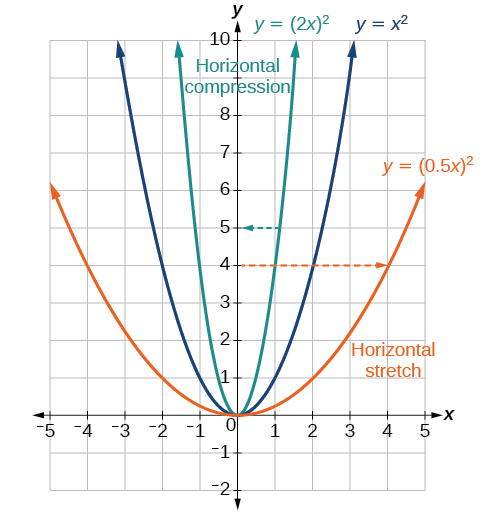
Figure 23
Given a function \(y = f(x),\) the form \(y = f(bx)\) results in a horizontal stretch or compression. Consider the function \(y = x^{2}.\) Observe Figure 23. The graph of \(y = \left( {0.5x} \right)^{2}\) is a horizontal stretch of the graph of the function \(y = x^{2}\) by a factor of 2. The graph of \(y = \left( {2x} \right)^{2}\) is a horizontal compression of the graph of the function \(y = x^{2}\) by a factor of \(2\).
Suppose a scientist is comparing a population of fruit flies to a population that progresses through its lifespan twice as fast as the original population. In other words, this new population, \(R,\) will progress in 1 hour the same amount as the original population does in 2 hours, and in 2 hours, it will progress as much as the original population does in 4 hours. Sketch a graph of this population.
Solution (click to reveal)
Symbolically, we could write
\[\begin{array}{rcl} {R(1)} & = & {P(2),} \\ {R(2)} & = & {P(4),\mspace{9mu}\text{and~in~general,}} \\ {R(t)} & = & {P(2t).} \end{array}\]
See Figure 24 for a graphical comparison of the original population and the compressed population.
![Two side-by-side graphs. The first graph has function for original population whose domain is [0,7] and range is [0,3]. The maximum value occurs at (3,3). The second graph has the same shape as the first except it is half as wide. It is a graph of transformed population, with a domain of [0, 3.5] and a range of [0,3]. The maximum occurs at (1.5, 3).](../images/CNX_Precalc_Figure_01_05_029ab.jpg)
Figure 24 (a) Original population graph (b) Compressed population graph
Note that the effect on the graph is a horizontal compression where all input values are half of their original distance from the vertical axis.
A function \(f(x)\) is given as Table 13. Create a table for the function \(g(x) = f\left( {\frac{1}{2}x} \right).\)
| \(x\) | 2 | 4 | 6 | 8 |
| \(f(x)\) | 1 | 3 | 7 | 11 |
Table 13
Solution (click to reveal)
The formula \(g(x) = f\left( {\frac{1}{2}x} \right)\) tells us that the output values for \(g\) are the same as the output values for the function \(f\) at an input half the size. Notice that we do not have enough information to determine \(g(2)\) because \(g(2) = f\left( {\frac{1}{2} \cdot 2} \right) = f(1),\) and we do not have a value for \(f(1)\) in our table. Our input values to \(g\) will need to be twice as large to get inputs for \(f\) that we can evaluate. For example, we can determine \(g(4)\text{.}\)
\[g(4) = f\left( {\frac{1}{2} \cdot 4} \right) = f(2) = 1\]
We do the same for the other values to produce Table 14.
| \(x\) | 4 | 8 | 12 | 16 |
| \(g(x)\) | 1 | 3 | 7 | 11 |
Table 14
Figure 25 shows the graphs of both of these sets of points.
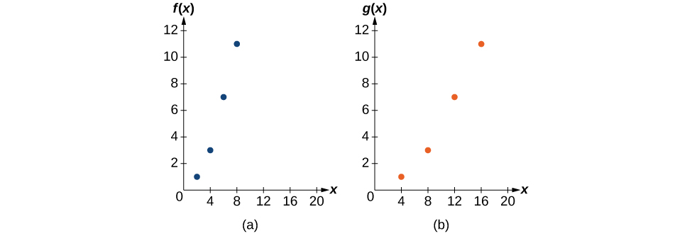
Figure 25
Because each input value has been doubled, the result is that the function \(g(x)\) has been stretched horizontally by a factor of 2.
Relate the function \(g(x)\) to \(f(x)\) in Figure 26.
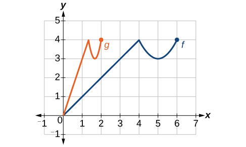
Figure 26
Solution (click to reveal)
The graph of \(g(x)\) looks like the graph of \(f(x)\) horizontally compressed. Because \(f(x)\) ends at \((6,4)\) and \(g(x)\) ends at \((2,4),\) we can see that the \(x\text{-}\) values have been compressed by \(\frac{1}{3},\) because \(6\left( \frac{1}{3} \right) = 2.\) We might also notice that \(g(2) = f(6)\) and \(g(1) = f(3).\) Either way, we can describe this relationship as \(g(x) = f\left( {3x} \right).\) This is a horizontal compression by \(\frac{1}{3}.\)
Notice that the coefficient needed for a horizontal stretch or compression is the reciprocal of the stretch or compression. So to stretch the graph horizontally by a scale factor of 4, we need a coefficient of \(\frac{1}{4}\) in our function: \(f\left( {\frac{1}{4}x} \right).\) This means that the input values must be four times larger to produce the same result, requiring the input to be larger, causing the horizontal stretching.
3.5.5 Performing a Sequence of Transformations
When combining transformations, it is very important to consider the order of the transformations. For example, vertically shifting by 3 and then vertically stretching by 2 does not create the same graph as vertically stretching by 2 and then vertically shifting by 3, because when we shift first, both the original function and the shift get stretched, while only the original function gets stretched when we stretch first.
When we see an expression such as \(2f(x) + 3,\) which transformation should we start with? The answer here follows nicely from the order of operations. Given the output value of \(f(x),\) we first multiply by 2, causing the vertical stretch, and then add 3, causing the vertical shift. In other words, multiplication before addition.
Horizontal transformations are a little trickier to think about. When we write \(g(x) = f(2x + 3),\) for example, we have to think about how the inputs to the function \(g\) relate to the inputs to the function \(f.\) Suppose we know \(f(7) = 12.\) What input to \(g\) would produce that output? In other words, what value of \(x\) will allow \(g(x) = f(2x + 3) = 12?\) We would need \(2x + 3 = 7.\) To solve for \(x,\) we would first subtract 3, resulting in a horizontal shift, and then divide by 2, causing a horizontal compression.
This format ends up being very difficult to work with, because it is usually much easier to horizontally stretch a graph before shifting. We can work around this by factoring inside the function.
\[f(bx + p) = f\left( {b\left( {x + \frac{p}{b}} \right)} \right)\]
Let’s work through an example.
\[f(x) = \left( {2x + 4} \right)^{2}\]
We can factor out a 2.
\[f(x) = \left( {2\left( {x + 2} \right)} \right)^{2}\]
Now we can more clearly observe a horizontal shift to the left 2 units and a horizontal compression. Factoring in this way allows us to horizontally stretch first and then shift horizontally.
Use the graph of \(f(x)\) in Figure 27 to sketch a graph of \(k(x) = f\left( {\frac{1}{2}x + 1} \right) - 3.\)
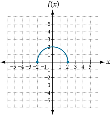
Figure 27
Solution (click to reveal)
To simplify, let’s start by factoring out the inside of the function.
\[f\left( {\frac{1}{2}x + 1} \right) - 3 = f\left( {\frac{1}{2}(x + 2)} \right) - 3\]
By factoring the inside, we can first horizontally stretch by 2, as indicated by the \(\frac{1}{2}\) on the inside of the function. Remember that twice the size of 0 is still 0, so the point (0,2) remains at (0,2) while the point (2,0) will stretch to (4,0). See Figure 28.
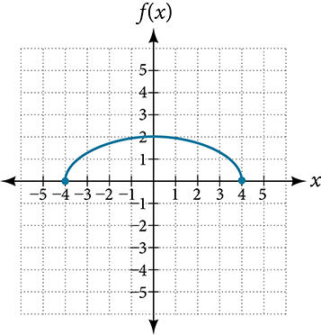
Figure 28
Next, we horizontally shift left by 2 units, as indicated by \(x + 2.\) See Figure 29.
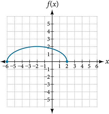
Figure 29
Last, we vertically shift down by 3 to complete our sketch, as indicated by the \(- 3\) on the outside of the function. See Figure 30.
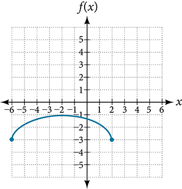
Figure 30
Section Exercises
Verbal
1. When examining the formula of a function that is the result of multiple transformations, how can you tell a horizontal shift from a vertical shift?
Solution (click to reveal)
A horizontal shift results when a constant is added to or subtracted from the input. A vertical shifts results when a constant is added to or subtracted from the output.
2. When examining the formula of a function that is the result of multiple transformations, how can you tell a horizontal stretch from a vertical stretch?
3. When examining the formula of a function that is the result of multiple transformations, how can you tell a horizontal compression from a vertical compression?
Solution (click to reveal)
A horizontal compression results when a constant greater than 1 is multiplied by the input. A vertical compression results when a constant between 0 and 1 is multiplied by the output.
4. When examining the formula of a function that is the result of multiple transformations, how can you tell a reflection with respect to the \(x\)-axis from a reflection with respect to the \(y\)-axis?
5. How can you determine whether a function is odd or even from the formula of the function?
Solution (click to reveal)
For a function \(f,\) substitute \(( - x)\) for \((x)\) in \(f(x).\) Simplify. If the resulting function is the same as the original function, \(f( - x) = f(x),\) then the function is even. If the resulting function is the opposite of the original function, \(f( - x) = - f(x),\) then the original function is odd. If the function is not the same or the opposite, then the function is neither odd nor even.
Algebraic
For the following exercises, write a formula for the function obtained when the graph is shifted as described.
6. \(f(x) = \sqrt{x}\) is shifted up 1 unit and to the left 2 units.
7. \(f(x) = |x|\) is shifted down 3 units and to the right 1 unit.
Solution (click to reveal)
\(\left. g(x) = \middle| x - 1 \middle| - 3 \right.\)
8. \(f(x) = \frac{1}{x}\) is shifted down 4 units and to the right 3 units.
9. \(f(x) = \frac{1}{x^{2}}\) is shifted up 2 units and to the left 4 units.
Solution (click to reveal)
\(g(x) = \frac{1}{{(x + 4)}^{2}} + 2\)
For the following exercises, describe how the graph of the function is a transformation of the graph of the original function \(f.\)
10. \(y = f(x - 49)\)
11. \(y = f(x + 43)\)
Solution (click to reveal)
The graph of \(f(x + 43)\) is a horizontal shift to the left 43 units of the graph of \(f.\)
12. \(y = f(x + 3)\)
13. \(y = f(x - 4)\)
Solution (click to reveal)
The graph of \(f(x - 4)\) is a horizontal shift to the right 4 units of the graph of \(f.\)
14. \(y = f(x) + 5\)
15. \(y = f(x) + 8\)
Solution (click to reveal)
The graph of \(f(x) + 8\) is a vertical shift up 8 units of the graph of \(f.\)
16. \(y = f(x) - 2\)
17. \(y = f(x) - 7\)
Solution (click to reveal)
The graph of \(f(x) - 7\) is a vertical shift down 7 units of the graph of \(f.\)
18. \(y = f(x - 2) + 3\)
19. \(y = f(x + 4) - 1\)
Solution (click to reveal)
The graph of \(f(x + 4) - 1\) is a horizontal shift to the left 4 units and a vertical shift down 1 unit of the graph of \(f.\)
For the following exercises, determine the interval(s) on which the function is increasing and decreasing.
20. \(f(x) = 4{(x + 1)}^{2} - 5\)
21. \(g(x) = 5{(x + 3)}^{2} - 2\)
Solution (click to reveal)
decreasing on \(( - \infty, - 3)\) and increasing on \(( - 3,\infty)\)
22. \(a(x) = \sqrt{- x + 4}\)
23. \(k(x) = - 3\sqrt{x} - 1\)
Solution (click to reveal)
decreasing on \((0,\mspace{9mu}\infty)\)
Graphical
For the following exercises, use the graph of \(f(x) = 2^{x}\) shown in Figure 31 to sketch a graph of each transformation of \(f(x).\)
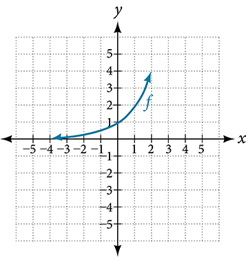
Figure 31
24. \(g(x) = 2^{x} + 1\)
25. \(h(x) = 2^{x} - 3\)
Solution (click to reveal)
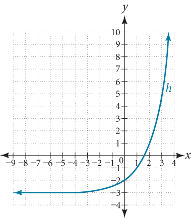
26. \(w(x) = 2^{x - 1}\)
For the following exercises, sketch a graph of the function as a transformation of the graph of one of the toolkit functions.
27. \(f(t) = {(t + 1)}^{2} - 3\)
Solution (click to reveal)
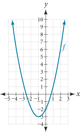
28. \(\left. h(x) = \middle| x - 1 \middle| + 4 \right.\)
29. \(k(x) = {(x - 2)}^{3} - 1\)
Solution (click to reveal)
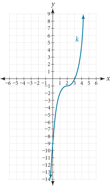
30. \(m(t) = 3 + \sqrt{t + 2}\)
Numeric
31. Tabular representations for the functions \(f,\mspace{9mu} g,\) and \(h\) are given below. Write \(g(x)\) and \(h(x)\) as transformations of \(f(x).\)
| \(x\) | −2 | −1 | 0 | 1 | 2 |
| \(f(x)\) | −2 | −1 | −3 | 1 | 2 |
| \(x\) | −1 | 0 | 1 | 2 | 3 |
| \(g(x)\) | −2 | −1 | −3 | 1 | 2 |
| \(x\) | −2 | −1 | 0 | 1 | 2 |
| \(h(x)\) | −1 | 0 | −2 | 2 | 3 |
Solution (click to reveal)
\(g(x) = f(x - 1),\mspace{9mu} h(x) = f(x) + 1\)
32. Tabular representations for the functions \(f,\mspace{9mu} g,\) and \(h\) are given below. Write \(g(x)\) and \(h(x)\) as transformations of \(f(x).\)
| \(x\) | −2 | −1 | 0 | 1 | 2 |
| \(f(x)\) | −1 | −3 | 4 | 2 | 1 |
| \(x\) | −3 | −2 | −1 | 0 | 1 |
| \(g(x)\) | −1 | −3 | 4 | 2 | 1 |
| \(x\) | −2 | −1 | 0 | 1 | 2 |
| \(h(x)\) | −2 | −4 | 3 | 1 | 0 |
For the following exercises, write an equation for each graphed function by using transformations of the graphs of one of the toolkit functions.
33.
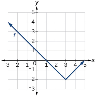
Solution (click to reveal)
\(\left. f(x) = \middle| x - 3 \middle| - 2 \right.\)
34.
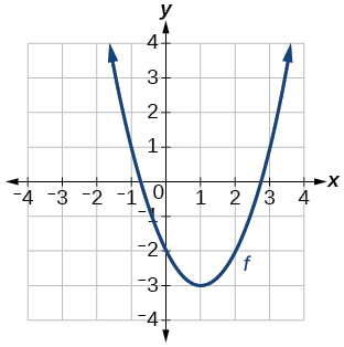
35.
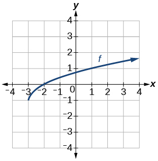
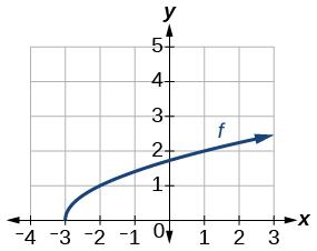
Solution (click to reveal)
\(f(x) = \sqrt{x + 3} - 1\)
36.
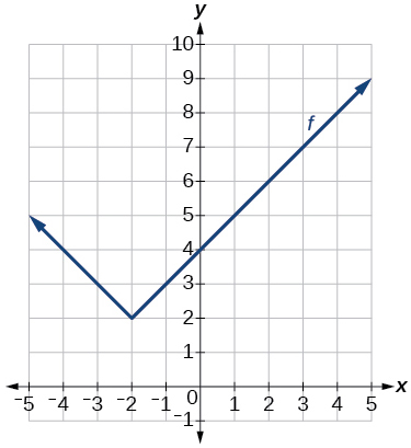
37.
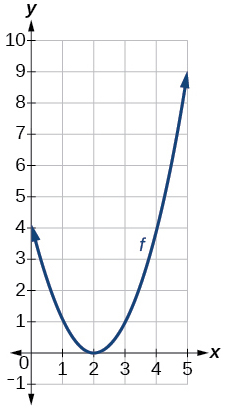
Solution (click to reveal)
\(f(x) = {(x - 2)}^{2}\)
38.
39.
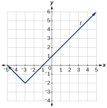
Solution (click to reveal)
\(\left. f(x) = \middle| x + 3 \middle| - 2 \right.\)
40.
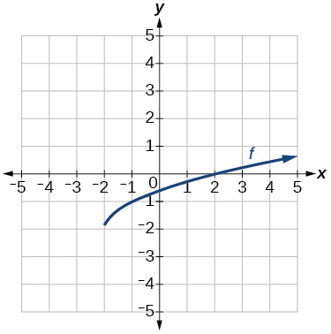
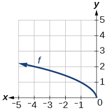
For the following exercises, use the graphs of transformations of the square root function to find a formula for each of the functions.
41.
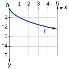
Solution (click to reveal)
\(f(x) = - \sqrt{x}\)
42.
For the following exercises, use the graphs of the transformed toolkit functions to write a formula for each of the resulting functions.
43.
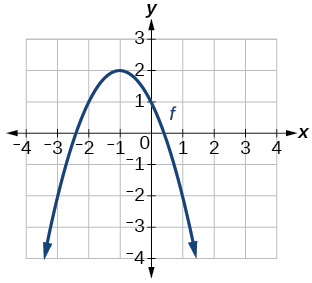
Solution (click to reveal)
\(f(x) = - {(x + 1)}^{2} + 2\)
44.
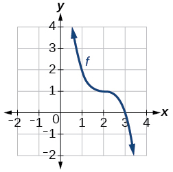
45.
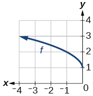
Solution (click to reveal)
\(f(x) = \sqrt{- x} + 1\)
46.
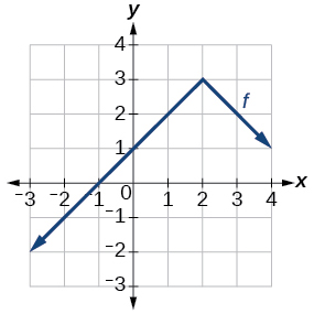
For the following exercises, determine whether the function is odd, even, or neither.
47. \(f(x) = 3x^{4}\)
Solution (click to reveal)
even
48. \(g(x) = \sqrt{x}\)
49. \(h(x) = \frac{1}{x} + 3x\)
Solution (click to reveal)
odd
50. \(f(x) = {(x - 2)}^{2}\)
51. \(g(x) = 2x^{4}\)
Solution (click to reveal)
even
52. \(h(x) = 2x - x^{3}\)
For the following exercises, describe how the graph of each function is a transformation of the graph of the original function \(f.\)
53. \(g(x) = - f(x)\)
Solution (click to reveal)
The graph of \(g\) is a vertical reflection (across the \(x\) -axis) of the graph of \(f.\)
54. \(g(x) = f( - x)\)
55. \(g(x) = 4f(x)\)
Solution (click to reveal)
The graph of \(g\) is a vertical stretch by a factor of 4 of the graph of \(f.\)
56. \(g(x) = 6f(x)\)
57. \(g(x) = f(5x)\)
Solution (click to reveal)
The graph of \(g\) is a horizontal compression by a factor of \(\frac{1}{5}\) of the graph of \(f.\)
58. \(g(x) = f(2x)\)
59. \(g(x) = f\left( {\frac{1}{3}x} \right)\)
Solution (click to reveal)
The graph of \(g\) is a horizontal stretch by a factor of 3 of the graph of \(f.\)
60. \(g(x) = f\left( {\frac{1}{5}x} \right)\)
61. \(g(x) = 3f\left( {- x} \right)\)
Solution (click to reveal)
The graph of \(g\) is a horizontal reflection across the \(y\) -axis and a vertical stretch by a factor of 3 of the graph of \(f.\)
62. \(g(x) = - f(3x)\)
For the following exercises, write a formula for the function \(g\) that results when the graph of a given toolkit function is transformed as described.
63. The graph of \(\left. f(x) = \middle| x \right|\) is reflected over the \(y\) -axis and horizontally compressed by a factor of \(\frac{1}{4}\) .
Solution (click to reveal)
\(\left. g(x) = \middle| - 4x \right|\)
64. The graph of \(f(x) = \sqrt{x}\) is reflected over the \(x\) -axis and horizontally stretched by a factor of 2.
65. The graph of \(f(x) = \frac{1}{x^{2}}\) is vertically compressed by a factor of \(\frac{1}{3},\) then shifted to the left 2 units and down 3 units.
Solution (click to reveal)
\(g(x) = \frac{1}{3{(x + 2)}^{2}} - 3\)
66. The graph of \(f(x) = \frac{1}{x}\) is vertically stretched by a factor of 8, then shifted to the right 4 units and up 2 units.
67. The graph of \(f(x) = x^{2}\) is vertically compressed by a factor of \(\frac{1}{2},\) then shifted to the right 5 units and up 1 unit.
Solution (click to reveal)
\(g(x) = \frac{1}{2}{(x - 5)}^{2} + 1\)
68. The graph of \(f(x) = x^{2}\) is horizontally stretched by a factor of 3, then shifted to the left 4 units and down 3 units.
For the following exercises, describe how the formula is a transformation of a toolkit function. Then sketch a graph of the transformation.
69. \(g(x) = 4{(x + 1)}^{2} - 5\)
Solution (click to reveal)
The graph of the function \(f(x) = x^{2}\) is shifted to the left 1 unit, stretched vertically by a factor of 4, and shifted down 5 units.
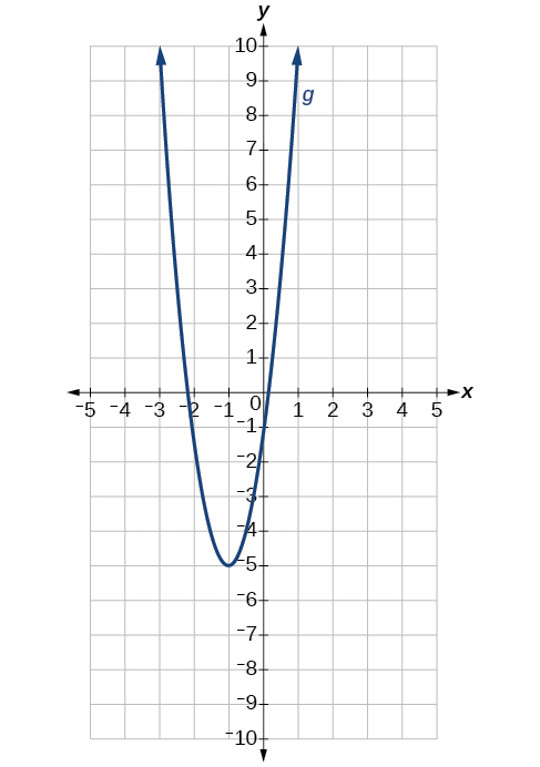
70. \(g(x) = 5{(x + 3)}^{2} - 2\)
71. \(\left. h(x) = - 2 \middle| x - 4 \middle| + 3 \right.\)
Solution (click to reveal)
The graph of \(\left. f(x) = \middle| x \right|\) is stretched vertically by a factor of 2, shifted horizontally 4 units to the right, reflected across the horizontal axis, and then shifted vertically 3 units up.
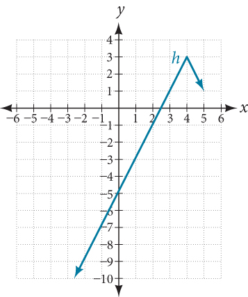
72. \(k(x) = - 3\sqrt{x} - 1\)
73. \(m(x) = \frac{1}{2}x^{3}\)
Solution (click to reveal)
The graph of the function \(f(x) = x^{3}\) is compressed vertically by a factor of \(\frac{1}{2}.\)
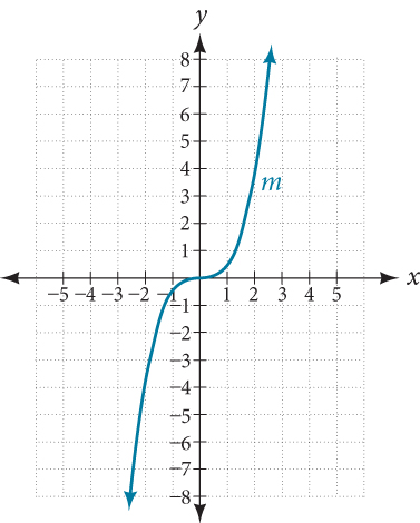
74. \(\left. n(x) = \frac{1}{3} \middle| x - 2 \right|\)
75. \(p(x) = \left( {\frac{1}{3}x} \right)^{3} - 3\)
Solution (click to reveal)
The graph of the function is stretched horizontally by a factor of 3 and then shifted vertically downward by 3 units.
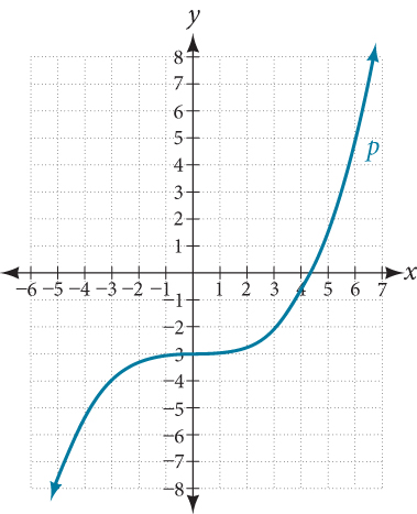
76. \(q(x) = \left( {\frac{1}{4}x} \right)^{3} + 1\)
77. \(a(x) = \sqrt{- x + 4}\)
Solution (click to reveal)
The graph of \(f(x) = \sqrt{x}\) is reflected across the \(y\)-axis and then shifted right 4 units.
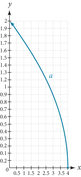
For the following exercises, use the graph in Figure 32 to sketch the given transformations.
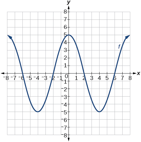
Figure 32
78. \(g(x) = f(x) - 2\)
79. \(g(x) = - f(x)\)
Solution (click to reveal)
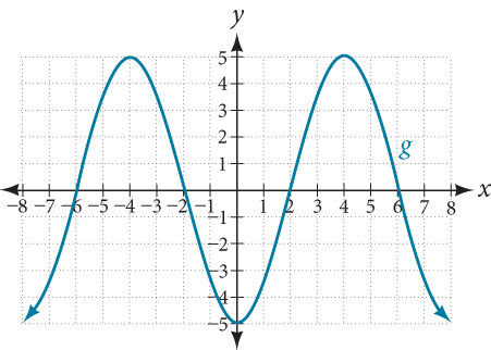
80. \(g(x) = f(x + 1)\)
81. \(g(x) = f(x - 2)\)
Solution (click to reveal)