5.3 Graphs of Polynomial Functions
The revenue in millions of dollars for a fictional cable company from 2006 through 2013 is shown in Table 1.
| Year | 2006 | 2007 | 2008 | 2009 | 2010 | 2011 | 2012 | 2013 |
| Revenues | 52.4 | 52.8 | 51.2 | 49.5 | 48.6 | 48.6 | 48.7 | 47.1 |
Table 1
The revenue can be modeled by the polynomial function
\[R(t) = - 0.037t^{4} + 1.414t^{3} - 19.777t^{2} + 118.696t - 205.332\]
where \(R\) represents the revenue in millions of dollars and \(t\) represents the year, with \(t = 6\) corresponding to 2006. Over which intervals is the revenue for the company increasing? Over which intervals is the revenue for the company decreasing? These questions, along with many others, can be answered by examining the graph of the polynomial function. We have already explored the local behavior of quadratics, a special case of polynomials. In this section we will explore the local behavior of polynomials in general.
5.3.1 Recognizing Characteristics of Graphs of Polynomial Functions
Polynomial functions of degree 2 or more have graphs that do not have sharp corners; recall that these types of graphs are called smooth curves. Polynomial functions also display graphs that have no breaks. Curves with no breaks are called continuous. Figure 1 shows a graph that represents a polynomial function and a graph that represents a function that is not a polynomial.
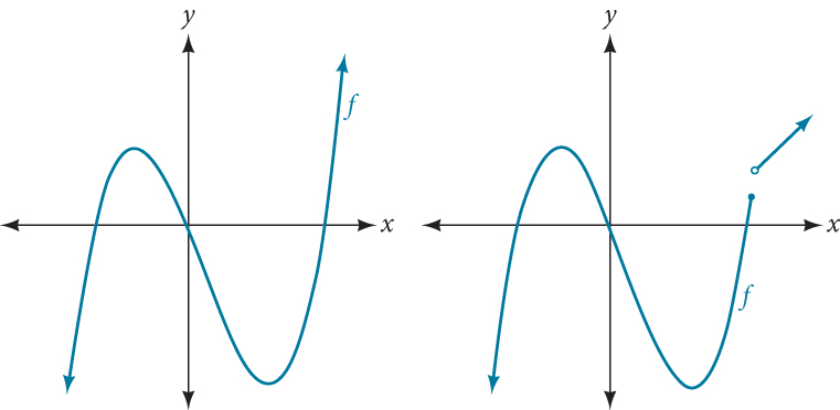
Figure 1
Which of the graphs in Figure 2 represents a polynomial function?
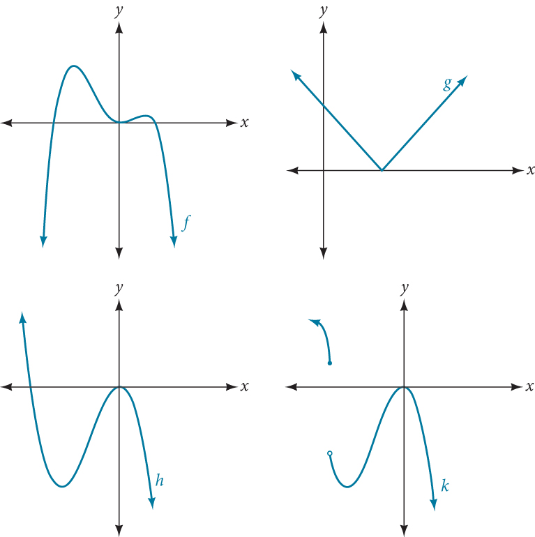
Figure 2
Solution (click to reveal)
The graphs of \(f\) and \(h\) are graphs of polynomial functions. They are smooth and continuous.
The graphs of \(g\) and \(k\) are graphs of functions that are not polynomials. The graph of function \(g\) has a sharp corner. The graph of function \(k\) is not continuous.
5.3.2 Using Factoring to Find Zeros of Polynomial Functions
Recall that if \(f\) is a polynomial function, the values of \(x\) for which \(f(x) = 0\) are called zeros of \(f.\) If the equation of the polynomial function can be factored, we can set each factor equal to zero and solve for the zeros.
We can use this method to find \(x\text{-}\) intercepts because at the \(x\text{-}\) intercepts we find the input values when the output value is zero. For general polynomials, this can be a challenging prospect. While quadratics can be solved using the relatively simple quadratic formula, the corresponding formulas for cubic and fourth-degree polynomials are not simple enough to remember, and formulas do not exist for general higher-degree polynomials. Consequently, we will limit ourselves to three cases:
- The polynomial can be factored using known methods: greatest common factor and trinomial factoring.
- The polynomial is given in factored form.
- Technology is used to determine the intercepts.
Find the \(x\)-intercepts of \(f(x) = x^{6} - 3x^{4} + 2x^{2}.\)
Solution (click to reveal)
We can attempt to factor this polynomial to find solutions for \(f(x) = 0.\)
\[\begin{array}{rclc} {x^{6} - 3x^{4} + 2x^{2}} & = & 0 & {\qquad\begin{array}{l} \text{Factor~out~the~greatest} \\ {\text{common~factor}\text{.}} \end{array}} \\ {x^{2}\left( x^{4} - 3x^{2} + 2 \right)} & = & 0 & {\qquad\text{Factor~the~trinomial}\text{.}} \\ {x^{2}\left( x^{2} - 1 \right)\left( x^{2} - 2 \right)} & = & 0 & {\qquad\text{Set~each~factor~equal~to~zero}\text{.}} \end{array}\]
\[\begin{array}{ccccrclcrcl} & & & & \left( x^{2} - 1 \right) & = & 0 & & \left( x^{2} - 2 \right) & = & 0 \\ x^{2} & = & 0 & {\qquad\text{or}} & x^{2} & = & 1 & {\qquad\text{or}} & x^{2} & = & 2 \\ x & = & 0 & & x & = & \pm 1 & & x & = & {\pm \sqrt{2}} \end{array}\]
This gives us five \(x\)-intercepts: \((0,0),(1,0),(-1,0),(\sqrt{2},0),\) and \(( - \sqrt{2},0).\) See Figure 3. We can see that this is an even function because it is symmetric about the \(y\)-axis.
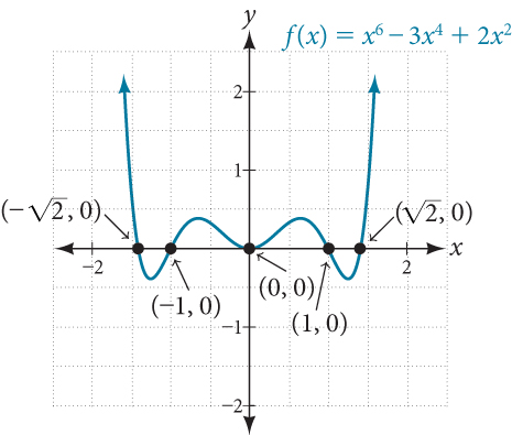
Figure 3
Find the \(x\)-intercepts of \(f(x) = x^{3} - 5x^{2} - x + 5.\)
Solution (click to reveal)
Find solutions for \(f(x) = 0\) by factoring.
\[\begin{array}{rcll} {x^{3} - 5x^{2} - x + 5} & = & 0 & {\qquad\text{Factor~by~grouping}\text{.}} \\ {x^{2}(x - 5) - (x - 5)} & = & 0 & {\qquad\text{Factor~out~the~common~factor}\text{.}} \\ {\left( x^{2} - 1 \right)(x - 5)} & = & 0 & {\qquad\text{Factor~the~difference~of~squares}\text{.}} \\ {(x + 1)(x - 1)(x - 5)} & = & 0 & {\qquad\text{Set~each~factor~equal~to~zero}\text{.}} \end{array}\]
\[\begin{array}{rclcrclcrcl} {x + 1} & = & 0 & {\qquad\text{or}\qquad} & {x - 1} & = & 0 & {\qquad\text{or}\qquad} & {x - 5} & = & 0 \\ x & = & -1 & & x & = & 1 & & x & = & 5 \end{array}\]
There are three \(x\)-intercepts: \((-1,0),(1,0),\) and \(\left( {5,0} \right).\) See Figure 4.
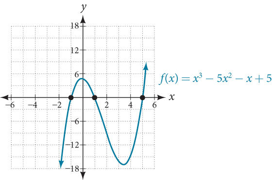
Figure 4
Find the \(y\)- and \(x\)-intercepts of \(g(x) = {(x - 2)}^{2}(2x + 3).\)
Solution (click to reveal)
The \(y\)-intercept can be found by evaluating \(g(0).\)
\[\begin{array}{ccl} {g(0)} & = & {{(0 - 2)}^{2}(2(0) + 3)} \\ & = & 12 \end{array}\]
So the \(y\)-intercept is \((0,12).\)
The \(x\)-intercepts can be found by solving \(g(x) = 0.\)
\[{(x - 2)}^{2}(2x + 3) = 0\]
\[\begin{array}{rclcccc} {(x - 2)}^{2} & = & 0 & & {(2x + 3)} & = & 0 \\ {x - 2} & = & 0 & {\qquad\text{or}\qquad} & x & = & {- \frac{3}{2}} \\ x & = & 2 & & & & \end{array}\]
So the \(x\)-intercepts are \((2,0)\) and \(\left( {- \frac{3}{2},0} \right).\)
We can always check that our answers are reasonable by using a graphing calculator to graph the polynomial as shown in Figure 5.
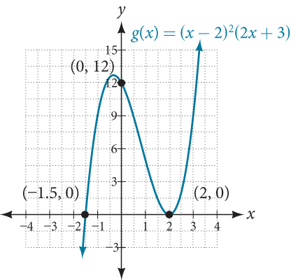
Figure 5
Find the \(x\)-intercepts of \(h(x) = x^{3} + 4x^{2} + x - 6.\)
Solution (click to reveal)
This polynomial is not in factored form, has no common factors, and does not appear to be factorable using techniques previously discussed. Fortunately, we can use technology to find the intercepts. Keep in mind that some values make graphing difficult by hand. In these cases, we can take advantage of graphing utilities.
Looking at the graph of this function, as shown in Figure 6, it appears that there are \(x\)-intercepts at \(x = -3,-2,\) and \(1.\)
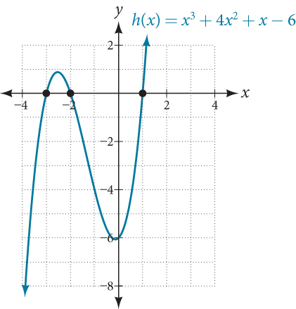
Figure 6
We can check whether these are correct by substituting these values for \(x\) and verifying that
\[h( - 3) = h( - 2) = h(1) = 0\]
Since \(h(x) = x^{3} + 4x^{2} + x - 6,\) we have:
\[\begin{array}{rcl} {h(-3)} & = & {{(-3)}^{3} + 4{(-3)}^{2} + (-3) - 6 = -27 + 36 - 3 - 6 = 0} \\ {h(-2)} & = & {{(-2)}^{3} + 4{(-2)}^{2} + (-2) - 6 = -8 + 16 - 2 - 6 = 0} \\ {h(1)} & = & {{(1)}^{3} + 4{(1)}^{2} + (1) - 6 = 1 + 4 + 1 - 6 = 0} \end{array}\]
Each \(x\)-intercept corresponds to a zero of the polynomial function and each zero yields a factor, so we can now write the polynomial in factored form.
\[\begin{array}{ccl} {h(x)} & = & {x^{3} + 4x^{2} + x - 6} \\ & = & {(x + 3)(x + 2)(x - 1)} \end{array}\]
5.3.3 Identifying Zeros and Their Multiplicities
Graphs behave differently at various \(x\)-intercepts. Sometimes, the graph will cross over the horizontal axis at an intercept. Other times, the graph will touch the horizontal axis and “bounce” off.
Suppose, for example, we graph the function shown.
\[f(x) = (x + 3){(x - 2)}^{2}{(x + 1)}^{3}\]
Notice in Figure 7 that the behavior of the function at each of the \(x\)-intercepts is different.
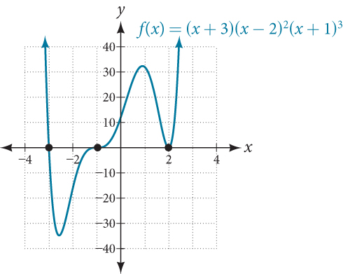
Figure 7 Identifying the behavior of the graph at an \(x\)-intercept by examining the multiplicity of the zero.
The \(x\)-intercept \(x = -3\) is the solution of equation \((x + 3) = 0.\) The graph passes directly through the \(x\)-intercept at \(x = -3.\) The factor is linear (has a degree of 1), so the behavior near the intercept is like that of a line—it passes directly through the intercept. We call this a single zero because the zero corresponds to a single factor of the function.
The \(x\)-intercept \(x = 2\) is the repeated solution of equation \({(x - 2)}^{2} = 0.\) The graph touches the axis at the intercept and changes direction. The factor is quadratic (degree 2), so the behavior near the intercept is like that of a quadratic—it bounces off of the horizontal axis at the intercept.
\[{(x - 2)}^{2} = (x - 2)(x - 2)\]
The factor is repeated, that is, the factor \(\left( {x - 2} \right)\) appears twice. The number of times a given factor appears in the factored form of the equation of a polynomial is called the multiplicity. The zero associated with this factor, \(x = 2,\) has multiplicity 2 because the factor \(\left( {x - 2} \right)\) occurs twice.
The \(x\)-intercept \(x = - 1\) is the repeated solution of factor \({(x + 1)}^{3} = 0.\) The graph passes through the axis at the intercept, but flattens out a bit first. This factor is cubic (degree 3), so the behavior near the intercept is like that of a cubic—with the same S-shape near the intercept as the toolkit function \(f(x) = x^{3}.\) We call this a triple zero, or a zero with multiplicity 3.
For zeros with even multiplicities, the graphs touch or are tangent to the \(x\)-axis. For zeros with odd multiplicities, the graphs cross or intersect the \(x\)-axis. See Figure 8 for examples of graphs of polynomial functions with multiplicity 1, 2, and 3.
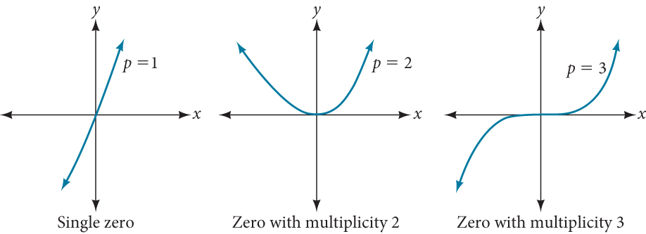
Figure 8
For higher even powers, such as 4, 6, and 8, the graph will still touch and bounce off of the horizontal axis but, for each increasing even power, the graph will appear flatter as it approaches and leaves the \(x\)-axis.
For higher odd powers, such as 5, 7, and 9, the graph will still cross through the horizontal axis, but for each increasing odd power, the graph will appear flatter as it approaches and leaves the \(x\)-axis.
Use the graph of the function of degree 6 in Figure 9 to identify the zeros of the function and their possible multiplicities.
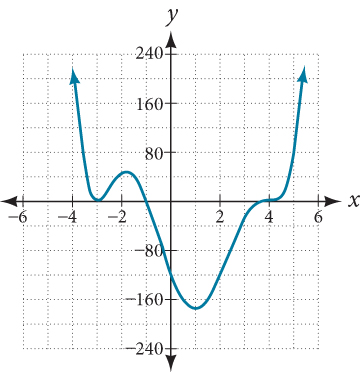
Figure 9
Solution (click to reveal)
The polynomial function is of degree 6. The sum of the multiplicities must be 6.
Starting from the left, the first zero occurs at \(x = -3.\) The graph touches the \(x\)-axis, so the multiplicity of the zero must be even. The zero of \(-3\) most likely has multiplicity \(2.\)
The next zero occurs at \(x = -1.\) The graph looks almost linear at this point. This is a single zero of multiplicity 1.
The last zero occurs at \(x = 4.\) The graph crosses thex-axis, so the multiplicity of the zero must be odd. We know that the multiplicity is likely 3 and that the sum of the multiplicities is 6.
Use the graph of the function of degree 9 in Figure 10 to identify the zeros of the function and their multiplicities.
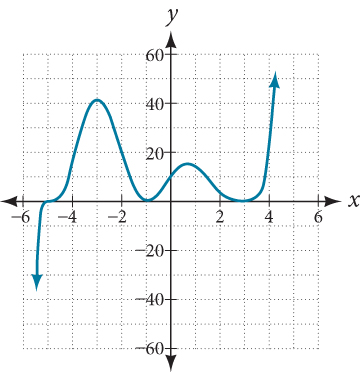
Figure 10
Solution (click to reveal)
The graph has a zero of –5 with multiplicity 3, a zero of -1 with multiplicity 2, and a zero of 3 with multiplicity 4.
5.3.4 Determining End Behavior
As we have already learned, the behavior of a graph of a polynomial function of the form
\[f(x) = a_{n}x^{n} + a_{n - 1}x^{n - 1} + ... + a_{1}x + a_{0}\]
will either ultimately rise or fall as \(x\) increases without bound and will either rise or fall as \(x\) decreases without bound. This is because for very large inputs, say 100 or 1,000, the leading term dominates the size of the output. The same is true for very small inputs, say –100 or –1,000.
Recall that we call this behavior the end behavior of a function. As we pointed out when discussing quadratic equations, when the leading term of a polynomial function, \(a_{n}x^{n},\) is an even power function, as \(x\) increases or decreases without bound, \(f(x)\) increases without bound. When the leading term is an odd power function, as \(x\) decreases without bound, \(f(x)\) also decreases without bound; as \(x\) increases without bound, \(f(x)\) also increases without bound. If the leading term is negative, it will change the direction of the end behavior. Figure 11 summarizes all four cases.
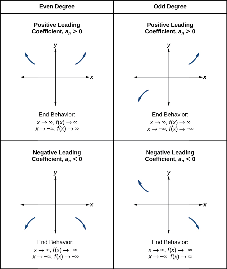
Figure 11
5.3.5 Understanding the Relationship between Degree and Turning Points
In addition to the end behavior, recall that we can analyze a polynomial function’s local behavior. It may have a turning point where the graph changes from increasing to decreasing (rising to falling) or decreasing to increasing (falling to rising). Look at the graph of the polynomial function \(f(x) = x^{4} - x^{3} - 4x^{2} + 4x\) in Figure 12. The graph has three turning points.
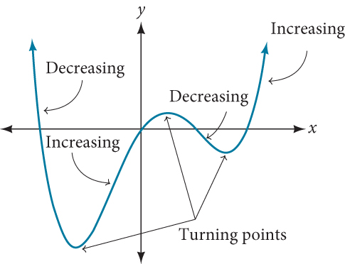
Figure 12
This function \(f\) is a 4th degree polynomial function and has 3 turning points. The maximum number of turning points of a polynomial function is always one less than the degree of the function.
Find the maximum number of turning points of each polynomial function.
ⓐ \(f(x) = - x^{3} + 4x^{5} - 3x^{2} + 1\)
ⓑ \(f(x) = - \left( {x - 1} \right)^{2}\left( {1 + 2x^{2}} \right)\)
Solution (click to reveal)
ⓐ First, rewrite the polynomial function in descending order: \(f(x) = 4x^{5} - x^{3} - 3x^{2} + 1\) Identify the degree of the polynomial function. This polynomial function is of degree 5. The maximum number of turning points is \(5 - 1 = 4.\)
ⓑ First, identify the leading term of the polynomial function if the function were expanded.

Then, identify the degree of the polynomial function. This polynomial function is of degree 4. The maximum number of turning points is \(4 - 1 = 3.\)
5.3.6 Graphing Polynomial Functions
We can use what we have learned about multiplicities, end behavior, and turning points to sketch graphs of polynomial functions. Let us put this all together and look at the steps required to graph polynomial functions.
Sketch a graph of \(f(x) = -2{(x + 3)}^{2}(x - 5).\)
Solution (click to reveal)
This graph has two \(x\)-intercepts. At \(x = -3,\) the factor is squared, indicating a multiplicity of 2. The graph will bounce at this \(x\)-intercept. At \(x = 5,\) the function has a multiplicity of one, indicating the graph will cross through the axis at this intercept.
The \(y\)-intercept is found by evaluating \(f(0).\)
\[\begin{array}{ccl} {f(0)} & = & {-2{(0 + 3)}^{2}(0 - 5)} \\ & = & {-2 \cdot 9 \cdot (-5)} \\ & = & 90 \end{array}\]
The \(y\)-intercept is \((0,90).\)
Additionally, we can see the leading term, if this polynomial were multiplied out, would be \(- 2x^{3},\) so the end behavior is that of a vertically reflected cubic, with the outputs decreasing as the inputs approach infinity, and the outputs increasing as the inputs approach negative infinity. See Figure 13.
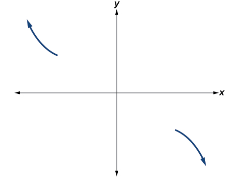
Figure 13
To sketch this, we consider that:
- As \(x\rightarrow - \infty\) the function \(f(x)\rightarrow\infty,\) so we know the graph starts in the second quadrant and is decreasing toward the \(x\text{-}\) axis.
- Since \(f\left( {- x} \right) = -2\left( {- x + 3} \right)^{2}\left( {- x–5} \right)\) is not equal to \(f(x),\) the graph does not display symmetry.
- At \(\left( {- 3,0} \right),\) the graph bounces off of the \(x\)-axis, so the function must start increasing.At \(\left( {0,90} \right),\) the graph crosses the \(y\)-axis at the \(y\)-intercept. See Figure 14.
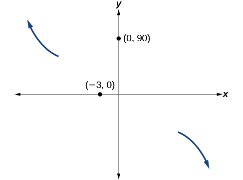
Figure 14
Somewhere after this point, the graph must turn back down or start decreasing toward the horizontal axis because the graph passes through the next intercept at \(\left( {5,0} \right).\) See Figure 15.
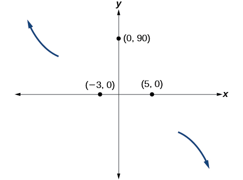
Figure 15
As \(x\rightarrow\infty\) the function \(f(x)\rightarrow{-\infty},\) so we know the graph continues to decrease, and we can stop drawing the graph in the fourth quadrant.
Using technology, we can create the graph for the polynomial function, shown in Figure 16, and verify that the resulting graph looks like our sketch in Figure 15.
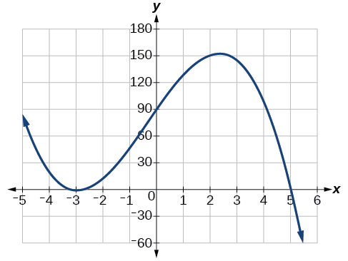
Figure 16 The complete graph of the polynomial function \(f(x) = - 2{(x + 3)}^{2}(x - 5)\)
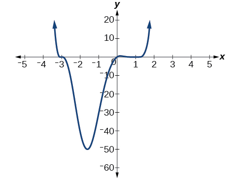
Sketch a graph of \(f(x) = \frac{1}{4}x{(x - 1)}^{4}{(x + 3)}^{3}.\)
Solution (click to reveal)
5.3.7 Using the Intermediate Value Theorem
In some situations, we may know two points on a graph but not the zeros. If those two points are on opposite sides of the \(x\)-axis, we can confirm that there is a zero between them. Consider a polynomial function \(f\) whose graph is smooth and continuous. The Intermediate Value Theorem states that for two numbers \(a\) and \(b\) in the domain of \(f,\) if \(a < b\) and \(f(a) \neq f(b),\) then the function \(f\) takes on every value between \(f(a)\) and \(f(b).\) (While the theorem is intuitive, the proof is actually quite complicated and requires higher mathematics.) We can apply this theorem to a special case that is useful in graphing polynomial functions. If a point on the graph of a continuous function \(f\) at \(x = a\) lies above the \(x\text{-}\) axis and another point at \(x = b\) lies below the \(x\text{-}\) axis, there must exist a third point between \(x = a\) and \(x = b\) where the graph crosses the \(x\text{-}\) axis. Call this point \(\left( {c,\mspace{9mu} f(c)} \right).\) This means that we are assured there is a solution \(c\) where \(f(c) = 0.\)
In other words, the Intermediate Value Theorem tells us that when a polynomial function changes from a negative value to a positive value, the function must cross the \(x\text{-}\) axis. Figure 17 shows that there is a zero between \(a\) and \(b.\)
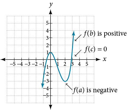
Figure 17 Using the Intermediate Value Theorem to show there exists a zero.
Show that the function \(f(x) = x^{3} - 5x^{2} + 3x + 6\) has at least two real zeros between \(x = 1\) and \(x = 4.\)
Solution (click to reveal)
As a start, evaluate \(f(x)\) at the integer values \(x = 1,2,3,\) and \(4.\) See Table 2.
| \(x\) | 1 | 2 | 3 | 4 |
| \(f(x)\) | 5 | 0 | –3 | 2 |
Table 2
We see that one zero occurs at \(x = 2.\) Also, since \(f(3)\) is negative and \(f(4)\) is positive, by the Intermediate Value Theorem, there must be at least one real zero between 3 and 4.
We have shown that there are at least two real zeros between \(x = 1\) and \(x = 4.\)
We can also see on the graph of the function in Figure 18 that there are two real zeros between \(x = 1\) and \(x = 4.\)
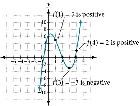
Figure 18
Writing Formulas for Polynomial Functions
Now that we know how to find zeros of polynomial functions, we can use them to write formulas based on graphs. Because a polynomial function written in factored form will have an \(x\)-intercept where each factor is equal to zero, we can form a function that will pass through a set of \(x\)-intercepts by introducing a corresponding set of factors.
Write a formula for the polynomial function shown in Figure 19.
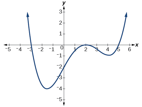
Figure 19
Solution (click to reveal)
This graph has three \(x\)-intercepts: \(x = -3,2,\) and \(5.\) The \(y\)-intercept is located at \((0, - 2).\) At \(x = -3\) and \(x = 5,\) the graph passes through the axis linearly, suggesting the corresponding factors of the polynomial will be linear. At \(x = 2,\) the graph bounces at the intercept, suggesting the corresponding factor of the polynomial will be second degree (quadratic). Together, this gives us
\[f(x) = a(x + 3){(x - 2)}^{2}(x - 5)\]
To determine the stretch factor, we utilize another point on the graph. We will use the \(y\text{-}\) intercept \((0,–2),\) to solve for \(a.\)
\[\begin{array}{rcl} {f(0)} & = & {a(0 + 3){(0 - 2)}^{2}(0 - 5)} \\ -2 & = & {a(0 + 3){(0 - 2)}^{2}(0 - 5)} \\ -2 & = & {- 60a} \\ a & = & \frac{1}{30} \end{array}\]
The graphed polynomial appears to represent the function \(f(x) = \frac{1}{30}(x + 3){(x - 2)}^{2}(x - 5).\)
Given the graph shown in Figure 20, write a formula for the function shown.
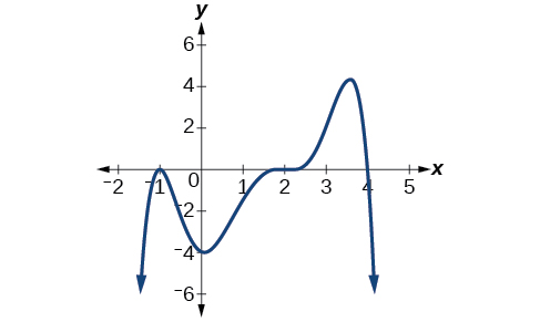
Figure 20
Solution (click to reveal)
\(f(x) = - \frac{1}{8}{(x - 2)}^{3}{(x + 1)}^{2}(x - 4)\)
Using Local and Global Extrema
With quadratics, we were able to algebraically find the maximum or minimum value of the function by finding the vertex. For general polynomials, finding these turning points is not possible without more advanced techniques from calculus. Even then, finding where extrema occur can still be algebraically challenging. For now, we will estimate the locations of turning points using technology to generate a graph.
Each turning point represents a local minimum or maximum. Sometimes, a turning point is the highest or lowest point on the entire graph. In these cases, we say that the turning point is a global maximum or a global minimum. These are also referred to as the absolute maximum and absolute minimum values of the function.
A local maximum or local minimum at \(x = a\) (sometimes called the relative maximum or minimum, respectively) is the output at the highest or lowest point on the graph in an open interval around \(x = a.\) If a function has a local maximum at \(a,\) then \(f(a) \geq f(x)\) for all \(x\) in an open interval around \(x = a.\) If a function has a local minimum at \(a,\) then \(f(a) \leq f(x)\) for all \(x\) in an open interval around \(x = a.\)
A global maximum or global minimum is the output at the highest or lowest point of the function. If a function has a global maximum at \(a,\) then \(f(a) \geq f(x)\) for all \(x.\) If a function has a global minimum at \(a,\) then \(f(a) \leq f(x)\) for all \(x.\)
We can see the difference between local and global extrema in Figure 21.
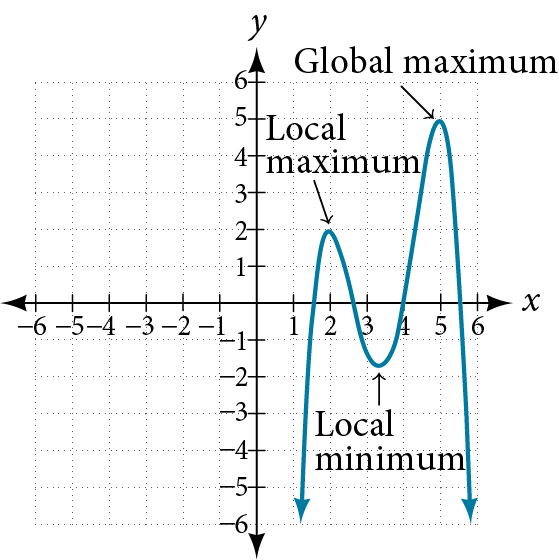
Figure 21
An open-top box is to be constructed by cutting out squares from each corner of a 14 cm by 20 cm sheet of plastic and then folding up the sides. Find the size of squares that should be cut out to maximize the volume enclosed by the box.
Solution (click to reveal)
We will start this problem by drawing a picture like that in Figure 22, labeling the width of the cut-out squares with a variable, \(w.\)
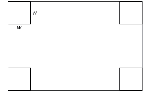
Figure 22
Notice that after a square is cut out from each end, it leaves a \(\left( {14 - 2w} \right)\) cm by \(\left( {20 - 2w} \right)\) cm rectangle for the base of the box, and the box will be \(w\) cm tall. This gives the volume
\[\begin{array}{ccl} {V(w)} & = & {(20 - 2w)(14 - 2w)w} \\ & = & {280w - 68w^{2} + 4w^{3}} \end{array}\]
Notice, since the factors are \(w,\) \(20–2w\) and \(14–2w,\) the three zeros are 10, 7, and 0, respectively. Because a height of 0 cm is not reasonable, we consider the only the zeros 10 and 7. The shortest side is 14 and we are cutting off two squares, so values \(w\) may take on are greater than zero or less than 7. This means we will restrict the domain of this function to \(0 < w < 7.\) Using technology to sketch the graph of \(V(w)\) on this reasonable domain, we get a graph like that in Figure 23. We can use this graph to estimate the maximum value for the volume, restricted to values for \(w\) that are reasonable for this problem—values from 0 to 7.
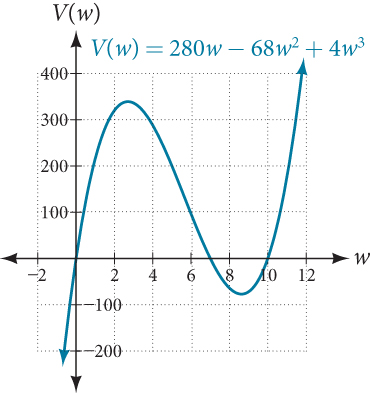
Figure 23
From this graph, we turn our focus to only the portion on the reasonable domain, \(\left\lbrack {0,\mspace{9mu} 7} \right\rbrack.\) We can estimate the maximum value to be around 340 cubic cm, which occurs when the squares are about 2.75 cm on each side. To improve this estimate, we could use advanced features of our technology, if available, or simply change our window to zoom in on our graph to produce Figure 24.
![Graph of V(w)=(20-2w)(14-2w)w where the x-axis is labeled w and the y-axis is labeled V(w) on the domain [2.4, 3].](../images/CNX_Precalc_Figure_03_04_029.jpg)
Figure 24
From this zoomed-in view, we can refine our estimate for the maximum volume to about 339 cubic cm, when the squares measure approximately 2.7 cm on each side.
Section Exercises
Verbal
1. What is the difference between an \(x\text{-}\) intercept and a zero of a polynomial function \(f?\)
Solution (click to reveal)
The \(x\text{-}\) intercept is where the graph of the function crosses the \(x\text{-}\) axis, and the zero of the function is the input value for which \(f(x) = 0.\)
2. If a polynomial function of degree \(n\) has \(n\) distinct zeros, what do you know about the graph of the function?
3. Explain how the Intermediate Value Theorem can assist us in finding a zero of a function.
Solution (click to reveal)
If we evaluate the function at \(a\) and at \(b\) and the sign of the function value changes, then we know a zero exists between \(a\) and \(b.\)
4. Explain how the factored form of the polynomial helps us in graphing it.
5. If the graph of a polynomial just touches the \(x\)-axis and then changes direction, what can we conclude about the factored form of the polynomial?
Solution (click to reveal)
There will be a factor raised to an even power.
Algebraic
For the following exercises, find the \(x\text{-}\) or \(t\)-intercepts of the polynomial functions.
6. \(C(t) = 2\left( {t - 4} \right)\left( {t + 1} \right)(t - 6)\)
7. \(C(t) = 3\left( {t + 2} \right)\left( {t - 3} \right)(t + 5)\)
Solution (click to reveal)
\(( - 2,0),(3,0),( - 5,0)\)
8. \(C(t) = 4t\left( {t - 2} \right)^{2}(t + 1)\)
9. \(C(t) = 2t\left( {t - 3} \right)\left( {t + 1} \right)^{2}\)
Solution (click to reveal)
\((3,0),( - 1,0),(0,0)\)
10. \(C(t) = 2t^{4} - 8t^{3} + 6t^{2}\)
11. \(C(t) = 4t^{4} + 12t^{3} - 40t^{2}\)
Solution (click to reveal)
\(\left( {0,0} \right),\mspace{9mu}\left( {- 5,0} \right),\mspace{9mu}\left( {2,0} \right)\)
12. \(f(x) = x^{4} - x^{2}\)
13. \(f(x) = x^{3} + x^{2} - 20x\)
Solution (click to reveal)
\(\left( {0,0} \right),\mspace{9mu}\left( {- 5,0} \right),\mspace{9mu}\left( {4,0} \right)\)
14. \(f(x) = x^{3} + 6x^{2} - 7x\)
15. \(f(x) = x^{3} + x^{2} - 4x - 4\)
Solution (click to reveal)
\(\left( {2,0} \right),\mspace{9mu}\left( {- 2,0} \right),\mspace{9mu}\left( {- 1,0} \right)\)
16. \(f(x) = x^{3} + 2x^{2} - 9x - 18\)
17. \(f(x) = 2x^{3} - x^{2} - 8x + 4\)
Solution (click to reveal)
\(( - 2,0),\mspace{9mu}(2,0),\mspace{9mu}\left( {\frac{1}{2},0} \right)\)
18. \(f(x) = x^{6} - 7x^{3} - 8\)
19. \(f(x) = 2x^{4} + 6x^{2} - 8\)
Solution (click to reveal)
\(\left( {1,0} \right),\mspace{9mu}\left( {- 1,0} \right)\)
20. \(f(x) = x^{3} - 3x^{2} - x + 3\)
21. \(f(x) = x^{6} - 2x^{4} - 3x^{2}\)
Solution (click to reveal)
\((0,0),\mspace{9mu}(\sqrt{3},0),\mspace{9mu}( - \sqrt{3},0)\)
22. \(f(x) = x^{6} - 3x^{4} - 4x^{2}\)
23. \(f(x) = x^{5} - 5x^{3} + 4x\)
Solution (click to reveal)
\(\left( {0,0} \right),\mspace{9mu}\left( {1,0} \right)\text{,~}\left( {- 1,0} \right),\mspace{9mu}\left( {2,0} \right),\mspace{9mu}\left( {- 2,0} \right)\)
For the following exercises, use the Intermediate Value Theorem to confirm that the given polynomial has at least one zero within the given interval.
24. \(f(x) = x^{3} - 9x,\) between \(x = -4\) and \(x = -2.\)
25. \(f(x) = x^{3} - 9x,\) between \(x = 2\) and \(x = 4.\)
Solution (click to reveal)
\(f(2) = –10\) and \(f(4) = 28.\) Sign change confirms.
26. \(f(x) = x^{5} - 2x,\) between \(x = 1\) and \(x = 2.\)
27. \(f(x) = - x^{4} + 4,\) between \(x = 1\) and \(x = 3\) .
Solution (click to reveal)
\(f(1) = 3\) and \(f(3) = –77.\) Sign change confirms.
28. \(f(x) = -2x^{3} - x,\) between \(x = –1\) and \(x = 1.\)
29. \(f(x) = x^{3} - 100x + 2,\) between \(x = 0.01\) and \(x = 0.1\)
Solution (click to reveal)
\(f(0.01) = 1.000001\) and \(f(0.1) = –7.999.\) Sign change confirms.
For the following exercises, find the zeros and give the multiplicity of each.
30. \(f(x) = \left( {x + 2} \right)^{3}\left( {x - 3} \right)^{2}\)
31. \(f(x) = x^{2}\left( {2x + 3} \right)^{5}\left( {x - 4} \right)^{2}\)
Solution (click to reveal)
0 with multiplicity 2, \(- \frac{3}{2}\) with multiplicity 5, 4 with multiplicity 2
32. \(f(x) = x^{3}\left( {x - 1} \right)^{3}\left( {x + 2} \right)\)
33. \(f(x) = x^{2}\left( {x^{2} + 4x + 4} \right)\)
Solution (click to reveal)
0 with multiplicity 2, –2 with multiplicity 2
34. \(f(x) = \left( {2x + 1} \right)^{3}\left( {9x^{2} - 6x + 1} \right)\)
35. \(f(x) = \left( {3x + 2} \right)^{5}\left( {x^{2} - 10x + 25} \right)\)
Solution (click to reveal)
\(- \frac{2}{3}\) with multiplicity 5, 5 with multiplicity 2
36. \(f(x) = x\left( {4x^{2} - 12x + 9} \right)\left( {x^{2} + 8x + 16} \right)\)
37. \(f(x) = x^{6} - x^{5} - 2x^{4}\)
Solution (click to reveal)
0 with multiplicity 4, 2 with multiplicity 1, −1 with multiplicity 1
38. \(f(x) = 3x^{4} + 6x^{3} + 3x^{2}\)
39. \(f(x) = 4x^{5} - 12x^{4} + 9x^{3}\)
Solution (click to reveal)
\(\frac{3}{2}\) with multiplicity 2, 0 with multiplicity 3
40. \(f(x) = 2x^{4}\left( {x^{3} - 4x^{2} + 4x} \right)\)
41. \(f(x) = 4x^{4}\left( {9x^{4} - 12x^{3} + 4x^{2}} \right)\)
Solution (click to reveal)
\(\text{0}\mspace{9mu}\text{with}\mspace{9mu}\text{multiplicity}\mspace{9mu} 6\text{,}\mspace{9mu}\frac{2}{3}\mspace{9mu}\text{with}\mspace{9mu}\text{multiplicity}\mspace{9mu} 2\)
Graphical
For the following exercises, graph the polynomial functions. Note \(x\text{-}\) and \(y\text{-}\) intercepts, multiplicity, and end behavior.
42. \(f(x) = \left( {x + 3} \right)^{2}(x - 2)\)
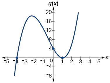
43. \(g(x) = \left( {x + 4} \right)\left( {x - 1} \right)^{2}\)
Solution (click to reveal)
\(x\)-intercepts, \((1,\ 0)\) with multiplicity 2, \(\left( {–4,~0} \right)\) with multiplicity 1, \(y\text{-}\) intercept \(\left( {0,~4}\operatorname{).} \right.\) As \(\ x\rightarrow - \infty,\ f(x)\rightarrow - \infty,\mspace{9mu}\text{as}\ x\rightarrow\infty,\ f(x)\rightarrow\infty.\)
44. \(h(x) = \left( {x - 1} \right)^{3}\left( {x + 3} \right)^{2}\)
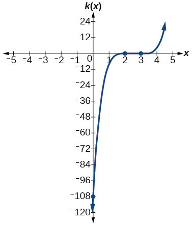
45. \(k(x) = \left( {x - 3} \right)^{3}\left( {x - 2} \right)^{2}\)
Solution (click to reveal)
\(x\)-intercepts \((3,0)\) with multiplicity 3, \((2,0)\) with multiplicity 2, \(y\text{-}\) intercept \((0,–108).\) As \(x\rightarrow - \infty,\ f(x)\rightarrow - \infty,\ \text{as}\ x\rightarrow\infty,\ f(x)\rightarrow\infty.\)
46. \(m(x) = - 2x\left( {x - 1} \right)(x + 3)\)
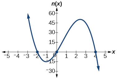
47. \(n(x) = - 3x\left( {x + 2} \right)(x - 4)\)
Solution (click to reveal)
\(x\)-intercepts \(\left( {0,~0} \right),\mspace{9mu}\left( {–2,~0} \right),\mspace{9mu}\left( {4,0} \right)\) with multiplicity 1, \(y\text{-}\) intercept \((0,~0).\) As \(x\rightarrow - \infty,\ f(x)\rightarrow\infty,\ \text{as}\ x\rightarrow\infty,\ f(x)\rightarrow - \infty.\)
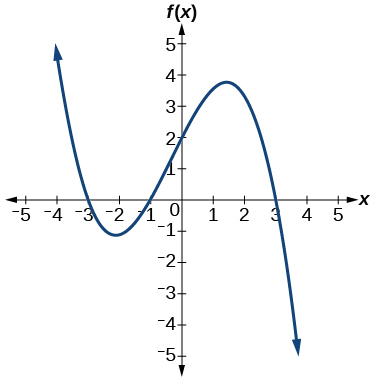
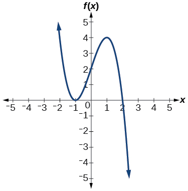
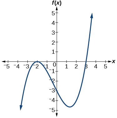
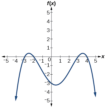
For the following exercises, use the graphs to write the formula for a polynomial function of least degree.
48.
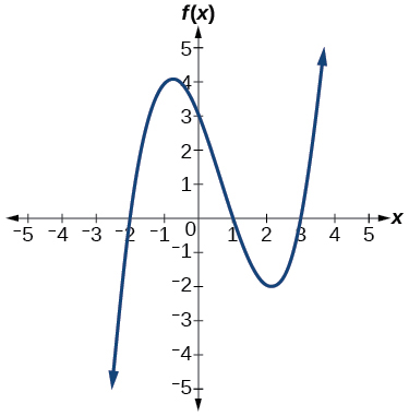
49.
Solution (click to reveal)
\(f(x) = - \frac{2}{9}(x - 3)(x + 1)(x + 3)\)
50.
51.
Solution (click to reveal)
\(f(x) = \frac{1}{4}{(x + 2)}^{2}(x - 3)\)
52.
For the following exercises, use the graph to identify zeros and multiplicity.
53.
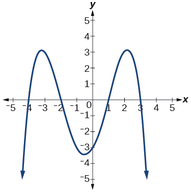
Solution (click to reveal)
–4, –2, 1, 3 with multiplicity 1
54.
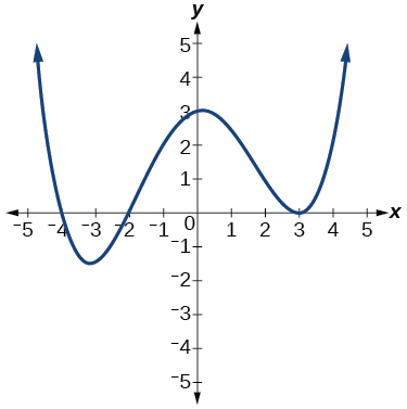
55.
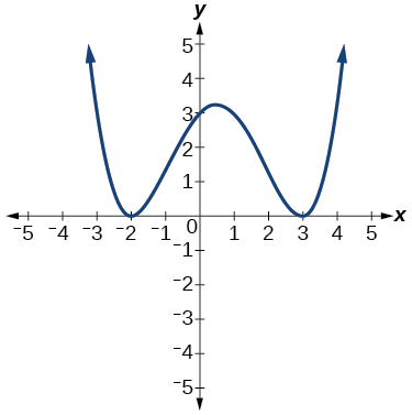
Solution (click to reveal)
–2, 3 each with multiplicity 2
56.
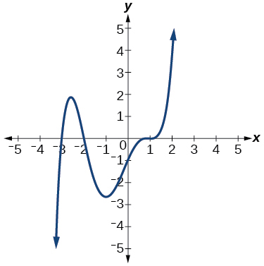
For the following exercises, use the given information about the polynomial graph to write the equation.
57. Degree 3. Zeros at \(x = –2,\) \(x = 1,\) and \(x = 3.\) \(y\)-intercept at \((0,–4).\)
Solution (click to reveal)
\(f(x) = - \frac{2}{3}(x + 2)(x - 1)(x - 3)\)
58. Degree 3. Zeros at \(x = \text{–5,}\) \(x = –2,\) and \(x = 1.\) \(y\)-intercept at \((0,6)\)
59. Degree 5. Roots of multiplicity 2 at \(x = 3\) and \(x = 1\) , and a root of multiplicity 1 at \(x = –3.\) \(y\)-intercept at \((0,9)\)
Solution (click to reveal)
\(f(x) = \frac{1}{3}{(x - 3)}^{2}{(x - 1)}^{2}(x + 3)\)
60. Degree 4. Root of multiplicity 2 at \(x = 4,\) and a roots of multiplicity 1 at \(x = 1\) and \(x = –2.\) \(y\)-intercept at \((0,\text{–}3).\)
61. Degree 5. Double zero at \(x = 1,\) and triple zero at \(x = 3.\) Passes through the point \((2,15).\)
Solution (click to reveal)
\(f(x) = -15{(x - 1)}^{2}{(x - 3)}^{3}\)
62. Degree 3. Zeros at \(x = 4,\) \(x = 3,\) and \(x = 2.\) \(y\)-intercept at \(\left( {0,-24} \right).\)
63. Degree 3. Zeros at \(x = -3,\) \(x = -2\) and \(x = 1.\) \(y\)-intercept at \((0,12).\)
Solution (click to reveal)
\(f(x) = - 2\left( {x + 3} \right)\left( {x + 2} \right)\left( {x - 1} \right)\)
64. Degree 5. Roots of multiplicity 2 at \(x = -3\) and \(x = 2\) and a root of multiplicity 1 at \(x = -2.\)
\(y\)-intercept at \(\left( {0,~4} \right).\)
65. Degree 4. Roots of multiplicity 2 at \(x = \frac{1}{2}\) and roots of multiplicity 1 at \(x = 6\) and \(x = -2.\)
\(y\)-intercept at \(\left( {0,18} \right).\)
Solution (click to reveal)
\(f(x) = - \frac{3}{2}\left( {2x - 1} \right)^{2}\left( {x - 6} \right)\left( {x + 2} \right)\)
66. Double zero at \(x = -3\) and triple zero at \(x = 0.\) Passes through the point \((1,32).\)
Technology
For the following exercises, use a calculator to approximate local minima and maxima or the global minimum and maximum.
67. \(f(x) = x^{3} - x - 1\)
Solution (click to reveal)
local max \(\left( {–\text{.58,~–}.62} \right),\) local min \(\left( {\text{.58,~–1}\text{.38}} \right)\)
68. \(f(x) = 2x^{3} - 3x - 1\)
69. \(f(x) = x^{4} + x\)
Solution (click to reveal)
global min \(\left( {–\text{.63,~–}\text{.47}} \right)\)
70. \(f(x) = - x^{4} + 3x - 2\)
71. \(f(x) = x^{4} - x^{3} + 1\)
Solution (click to reveal)
global min \(\text{(}\text{.75,~}\text{.89)}\)
Extensions
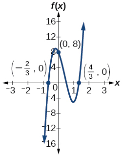
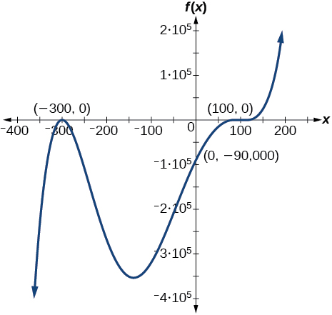
For the following exercises, use the graphs to write a polynomial function of least degree.
72.
73.
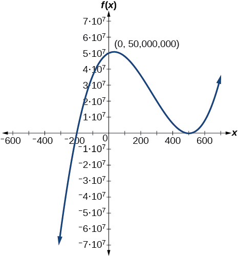
Solution (click to reveal)
\(f(x) = {(x - 500)}^{2}(x + 200)\)
74.
Real-World Applications
For the following exercises, write the polynomial function that models the given situation.
75. A rectangle has a length of 10 units and a width of 8 units. Squares of \(x\) by \(x\) units are cut out of each corner, and then the sides are folded up to create an open box. Express the volume of the box as a polynomial function in terms of \(x.\)
Solution (click to reveal)
\(f(x) = 4x^{3} - 36x^{2} + 80x\)
76. Consider the same rectangle of the preceding problem. Squares of \(2x\) by \(2x\) units are cut out of each corner. Express the volume of the box as a polynomial in terms of \(x.\)
77. A square has sides of 12 units. Squares \(x + 1\) by \(x + 1\) units are cut out of each corner, and then the sides are folded up to create an open box. Express the volume of the box as a function in terms of \(x.\)
Solution (click to reveal)
\(f(x) = 4x^{3} - 36x^{2} + 60x + 100\)
78. A cylinder has a radius of \(x + 2\) units and a height of 3 units greater. Express the volume of the cylinder as a polynomial function.
79. A right circular cone has a radius of \(3x + 6\) and a height 3 units less. Express the volume of the cone as a polynomial function. The volume of a cone is \(V = \frac{1}{3}\pi r^{2}h\) for radius \(r\) and height \(h.\)
Solution (click to reveal)
\(f(x) = 9\pi(x^{3} + 5x^{2} + 8x + 4)\)