6.8 Fitting Exponential Models to Data
In previous sections of this chapter, we were either given a function explicitly to graph or evaluate, or we were given a set of points that were guaranteed to lie on the curve. Then we used algebra to find the equation that fit the points exactly. In this section, we use a modeling technique called regression analysis to find a curve that models data collected from real-world observations. With regression analysis, we don’t expect all the points to lie perfectly on the curve. The idea is to find a model that best fits the data. Then we use the model to make predictions about future events.
Do not be confused by the word model. In mathematics, we often use the terms function, equation, and model interchangeably, even though they each have their own formal definition. The term model is typically used to indicate that the equation or function approximates a real-world situation.
We will concentrate on three types of regression models in this section: exponential, logarithmic, and logistic. Having already worked with each of these functions gives us an advantage. Knowing their formal definitions, the behavior of their graphs, and some of their real-world applications gives us the opportunity to deepen our understanding. As each regression model is presented, key features and definitions of its associated function are included for review. Take a moment to rethink each of these functions, reflect on the work we’ve done so far, and then explore the ways regression is used to model real-world phenomena.
6.8.1 Building an Exponential Model from Data
As we’ve learned, there are a multitude of situations that can be modeled by exponential functions, such as investment growth, radioactive decay, atmospheric pressure changes, and temperatures of a cooling object. What do these phenomena have in common? For one thing, all the models either increase or decrease as time moves forward. But that’s not the whole story. It’s the way data increase or decrease that helps us determine whether it is best modeled by an exponential equation. Knowing the behavior of exponential functions in general allows us to recognize when to use exponential regression, so let’s review exponential growth and decay.
Recall that exponential functions have the form \(y = ab^{x}\) or \(y = A_{0}e^{kx}.\) When performing regression analysis, we use the form most commonly used on graphing utilities, \(y = ab^{x}.\) Take a moment to reflect on the characteristics we’ve already learned about the exponential function \(y = ab^{x}\) (assume \(a > 0):\)
\(b\) must be greater than zero and not equal to one.
The initial value of the model is \(y = a.\)
If \(b > 1,\) the function models exponential growth. As \(x\) increases, the outputs of the model increase slowly at first, but then increase more and more rapidly, without bound.
If \(0 < b < 1,\) the function models exponential decay. As \(x\) increases, the outputs for the model decrease rapidly at first and then level off to become asymptotic to the \(x\)-axis. In other words, the outputs never become equal to or less than zero.
As part of the results, your calculator will display a number known as the correlation coefficient, labeled by the variable \(r,\) or \(r^{2}.\) (You may have to change the calculator’s settings for these to be shown.) The values are an indication of the “goodness of fit” of the regression equation to the data. We more commonly use the value of \(r^{2}\) instead of \(r,\) but the closer either value is to 1, the better the regression equation approximates the data.
In 2007, a university study was published investigating the crash risk of alcohol impaired driving. Data from 2,871 crashes were used to measure the association of a person’s blood alcohol level (BAC) with the risk of being in an accident. Table 1 shows results from the study . The relative risk is a measure of how many times more likely a person is to crash. So, for example, a person with a BAC of 0.09 is 3.54 times as likely to crash as a person who has not been drinking alcohol.
| BAC | 0 | 0.01 | 0.03 | 0.05 | 0.07 | 0.09 |
| Relative Risk of Crashing | 1 | 1.03 | 1.06 | 1.38 | 2.09 | 3.54 |
| BAC | 0.11 | 0.13 | 0.15 | 0.17 | 0.19 | 0.21 |
| Relative Risk of Crashing | 6.41 | 12.6 | 22.1 | 39.05 | 65.32 | 99.78 |
Table 1
- Let \(x\) represent the BAC level, and let \(y\) represent the corresponding relative risk. Use exponential regression to fit a model to these data.
- After 6 drinks, a person weighing 160 pounds will have a BAC of about \(0.16.\) How many times more likely is a person with this weight to crash if they drive after having a 6-pack of beer? Round to the nearest hundredth.
Solution (click to reveal)
- Using the STAT then EDIT menu on a graphing utility, list the BAC values in L1 and the relative risk values in L2. Then use the STATPLOT feature to verify that the scatterplot follows the exponential pattern shown in Figure 1:
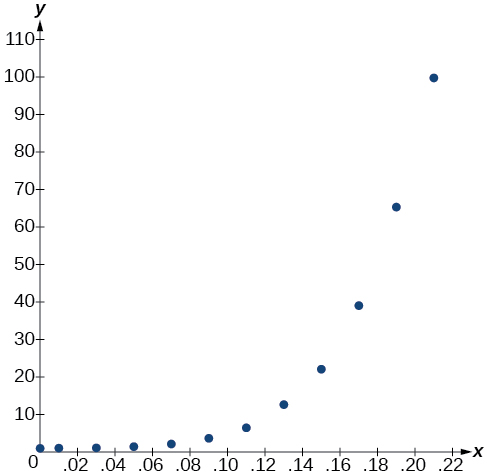
Figure 1
Use the “ExpReg” command from the STAT then CALC menu to obtain the exponential model,
\[y = 0.58304829\left( {2.20720213\text{E}10} \right)^{x}\]
Converting from scientific notation, we have:
\[y = 0.58304829\left( \text{22{,}072{,}021{,}300} \right)^{x}\]
Notice that \(r^{2} \approx 0.97\) which indicates the model is a good fit to the data. To see this, graph the model in the same window as the scatterplot to verify it is a good fit as shown in Figure 2:
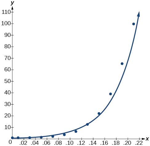
Figure 2
- Use the model to estimate the risk associated with a BAC of \(0.16.\) Substitute \(0.16\) for \(x\) in the model and solve for \(y.\)
\[\begin{array}{lll} y & {= 0.58304829\left( \text{22{,}072{,}021{,}300} \right)^{x}} & {\text{Use~the~regression~model~found~in~part~(a)}\text{.}} \\ & {= 0.58304829\left( \text{22{,}072{,}021{,}300} \right)^{0.16}} & {\text{Substitute~0}\text{.16~for~}x\text{.}} \\ & {\approx \text{26}\text{.35}} & {\text{Round~to~the~nearest~hundredth}\text{.}} \end{array}\]
If a 160-pound person drives after having 6 drinks, they are about 26.35 times more likely to crash than if driving while sober.
6.8.2 Building a Logarithmic Model from Data
Just as with exponential functions, there are many real-world applications for logarithmic functions: intensity of sound, pH levels of solutions, yields of chemical reactions, production of goods, and growth of infants. As with exponential models, data modeled by logarithmic functions are either always increasing or always decreasing as time moves forward. Again, it is the way they increase or decrease that helps us determine whether a logarithmic model is best.
Recall that logarithmic functions increase or decrease rapidly at first, but then steadily slow as time moves on. By reflecting on the characteristics we’ve already learned about this function, we can better analyze real world situations that reflect this type of growth or decay. When performing logarithmic regression analysis, we use the form of the logarithmic function most commonly used on graphing utilities, \(y = a + b\ln(x).\) For this function
- All input values, \(x,\) must be greater than zero.
- The point \(\left( {1,a} \right)\) is on the graph of the model.
- If \(b > 0,\) the model is increasing. Growth increases rapidly at first and then steadily slows over time.
- If \(b < 0,\) the model is decreasing. Decay occurs rapidly at first and then steadily slows over time.
Due to advances in medicine and higher standards of living, life expectancy has been increasing in most developed countries since the beginning of the 20th century.
Table 3 shows the average life expectancies, in years, of Americans from 1900–2010.
| Year | 1900 | 1910 | 1920 | 1930 | 1940 | 1950 |
| Life Expectancy(Years) | 47.3 | 50.0 | 54.1 | 59.7 | 62.9 | 68.2 |
| Year | 1960 | 1970 | 1980 | 1990 | 2000 | 2010 |
| Life Expectancy(Years) | 69.7 | 70.8 | 73.7 | 75.4 | 76.8 | 78.7 |
Table 3
ⓐ Let \(x\) represent time in decades starting with \(x = 1\) for the year 1900, \(x = 2\) for the year 1910, and so on. Let \(y\) represent the corresponding life expectancy. Use logarithmic regression to fit a model to these data.
ⓑ Use the model to predict the average American life expectancy for the year 2030.
Solution (click to reveal)
ⓐ Using the STAT then EDIT menu on a graphing utility, list the years using values 1–12 in L1 and the corresponding life expectancy in L2. Then use the STATPLOT feature to verify that the scatterplot follows a logarithmic pattern as shown in Figure 3:
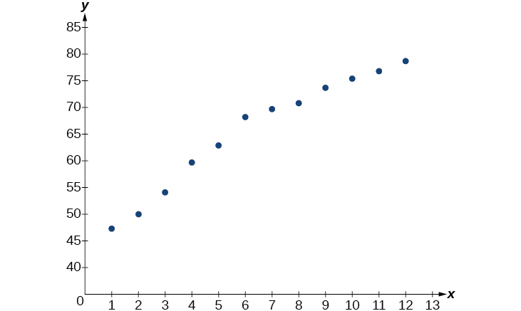
Figure 3
Use the “LnReg” command from the STAT then CALC menu to obtain the logarithmic model,
\[y = 42.52722583 + 13.85752327\ln(x)\]
Next, graph the model in the same window as the scatterplot to verify it is a good fit as shown in Figure 4:
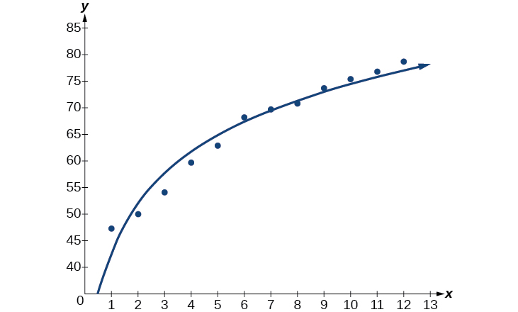
Figure 4
ⓑ To predict the life expectancy of an American in the year 2030, substitute \(x = 14\) for the in the model and solve for \(y:\)
\[\begin{array}{lll} y & {= 42.52722583 + 13.85752327\ln(x)} & {\text{Use~the~regression~model~found~in~part~(a)}\text{.}} \\ & {= 42.52722583 + 13.85752327\ln(14)} & {\text{Substitute~14~for~}x\text{.}} \\ & {\approx \text{79}\text{.1}} & \text{Round~to~the~nearest~tenth.} \end{array}\]
If life expectancy continues to increase at this pace, the average life expectancy of an American will be 79.1 by the year 2030.
6.8.3 Building a Logistic Model from Data
Like exponential and logarithmic growth, logistic growth increases over time. One of the most notable differences with logistic growth models is that, at a certain point, growth steadily slows and the function approaches an upper bound, or limiting value. Because of this, logistic regression is best for modeling phenomena where there are limits in expansion, such as availability of living space or nutrients.
It is worth pointing out that logistic functions actually model resource-limited exponential growth. There are many examples of this type of growth in real-world situations, including population growth and spread of disease, rumors, and even stains in fabric. When performing logistic regression analysis, we use the form most commonly used on graphing utilities:
\[y = \frac{c}{1 + ae^{- bx}}\]
Recall that:
- \(\frac{c}{1 + a}\) is the initial value of the model.
- when \(b > 0,\) the model increases rapidly at first until it reaches its point of maximum growth rate, \(\left( {\frac{\ln(a)}{b},\frac{c}{2}} \right).\) At that point, growth steadily slows and the function becomes asymptotic to the upper bound \(y = c.\)
- \(c\) is the limiting value, sometimes called the carrying capacity, of the model.
Mobile telephone service has increased rapidly in America since the mid 1990s. Today, almost all residents have cellular service. Table 5 shows the percentage of Americans with cellular service between the years 1995 and 2012 .
| Year | Americans with Cellular Service (%) | Year | Americans with Cellular Service (%) |
|---|---|---|---|
| 1995 | 12.69 | 2004 | 62.852 |
| 1996 | 16.35 | 2005 | 68.63 |
| 1997 | 20.29 | 2006 | 76.64 |
| 1998 | 25.08 | 2007 | 82.47 |
| 1999 | 30.81 | 2008 | 85.68 |
| 2000 | 38.75 | 2009 | 89.14 |
| 2001 | 45.00 | 2010 | 91.86 |
| 2002 | 49.16 | 2011 | 95.28 |
| 2003 | 55.15 | 2012 | 98.17 |
Table 5
- ⓐ Let \(x\) represent time in years starting with \(x = 0\) for the year 1995. Let \(y\) represent the corresponding percentage of residents with cellular service. Use logistic regression to fit a model to these data.
- ⓑ Use the model to calculate the percentage of Americans with cell service in the year 2013. Round to the nearest tenth of a percent.
- ⓒ Discuss the value returned for the upper limit, \(c.\) What does this tell you about the model? What would the limiting value be if the model were exact?
Solution (click to reveal)
- ⓐ Using the STAT then EDIT menu on a graphing utility, list the years using values 0–15 in L1 and the corresponding percentage in L2. Then use the STATPLOT feature to verify that the scatterplot follows a logistic pattern as shown in Figure 5:
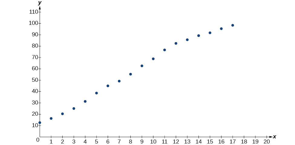
Figure 5
Use the “Logistic” command from the STAT then CALC menu to obtain the logistic model,
\[y = \frac{105.7379526}{1 + 6.88328979e^{- 0.2595440013x}}\]
Next, graph the model in the same window as shown in Figure 6 the scatterplot to verify it is a good fit:
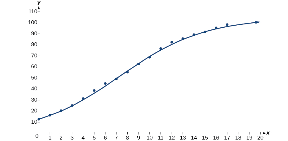
Figure 6
- ⓑ To approximate the percentage of Americans with cellular service in the year 2013, substitute \(x = 18\) for the in the model and solve for \(y:\)
\[\begin{array}{lll} y & {= \frac{105.7379526}{1 + 6.88328979e^{- 0.2595440013x}}} & {\text{Use~the~regression~model~found~in~part~(a)}.} \\ & {= \frac{105.7379526}{1 + 6.88328979e^{- 0.2595440013(18)}}} & {\text{Substitute~18~for~}x.} \\ & {\approx \text{99}\text{.3~}} & \text{Round~to~the~nearest~tenth} \end{array}\]
According to the model, about 99.3% of Americans had cellular service in 2013.
- ⓒ The model gives a limiting value of about 105. This means that the maximum possible percentage of Americans with cellular service would be 105%, which is impossible. (How could over 100% of a population have cellular service?) If the model were exact, the limiting value would be \(c = 100\) and the model’s outputs would get very close to, but never actually reach 100%. After all, there will always be someone out there without cellular service!
Section Exercises
Verbal
1. What situations are best modeled by a logistic equation? Give an example, and state a case for why the example is a good fit.
Solution (click to reveal)
Logistic models are best used for situations that have limited values. For example, populations cannot grow indefinitely since resources such as food, water, and space are limited, so a logistic model best describes populations.
2. What is a carrying capacity? What kind of model has a carrying capacity built into its formula? Why does this make sense?
3. What is regression analysis? Describe the process of performing regression analysis on a graphing utility.
Solution (click to reveal)
Regression analysis is the process of finding an equation that best fits a given set of data points. To perform a regression analysis on a graphing utility, first list the given points using the STAT then EDIT menu. Next graph the scatter plot using the STAT PLOT feature. The shape of the data points on the scatter graph can help determine which regression feature to use. Once this is determined, select the appropriate regression analysis command from the STAT then CALC menu.
4. What might a scatterplot of data points look like if it were best described by a logarithmic model?
5. What does the \(y\)-intercept on the graph of a logistic equation correspond to for a population modeled by that equation?
Solution (click to reveal)
The \(y\)-intercept on the graph of a logistic equation corresponds to the initial population for the population model.
Graphical
For the following exercises, match the given function of best fit with the appropriate scatterplot in Figure 7 through Figure 11. Answer using the letter beneath the matching graph.
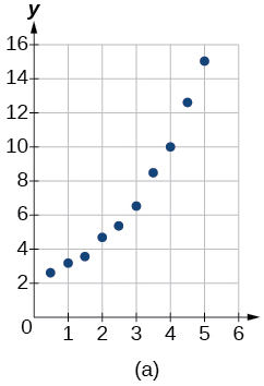
Figure 7
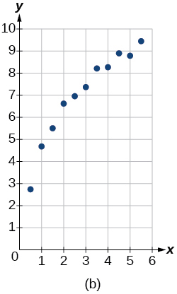
Figure 8
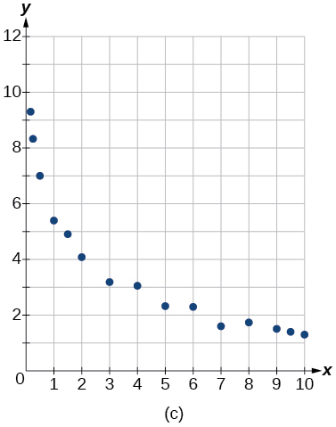
Figure 9
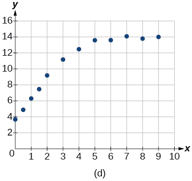
Figure 10
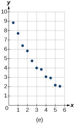
Figure 11
6. \(y = 10.209e^{- 0.294x}\)
7. \(y = 5.598 - 1.912\ln(x)\)
Solution (click to reveal)
C
8. \(y = 2.104(1.479)^{x}\)
9. \(y = 4.607 + 2.733\ln(x)\)
Solution (click to reveal)
B
10. \(y = \frac{14.005}{1 + 2.79e^{- 0.812x}}\)
Numeric
11. To the nearest whole number, what is the initial value of a population modeled by the logistic equation \(P(t) = \frac{175}{1 + 6.995e^{- 0.68t}}?\) What is the carrying capacity?
Solution (click to reveal)
\(P(0) = 22\) ; 175
12. Rewrite the exponential model \(A(t) = 1550(1.085)^{x}\) as an equivalent model with base \(e.\) Express the exponent to four significant digits.
13. A logarithmic model is given by the equation \(h(p) = 67.682 - 5.792\ln(p).\) To the nearest hundredth, for what value of \(p\) does \(h(p) = 62?\)
Solution (click to reveal)
\(p \approx 2.67\)
14. A logistic model is given by the equation \(P(t) = \frac{90}{1 + 5e^{- 0.42t}}.\) To the nearest hundredth, for what value of \(t\) does \(P(t) = 45?\)
15. What is the \(y\)-intercept on the graph of the logistic model given in the previous exercise?
Solution (click to reveal)
\(y\)-intercept: \(\left( {0,15} \right)\)
Technology
For the following exercises, use this scenario: The population \(P\) of a koi pond over \(x\) months is modeled by the function \(P(x) = \frac{68}{1 + 16e^{- 0.28x}}.\)
16. Graph the population model to show the population over a span of \(3\) years.
17. What was the initial population of koi?
Solution (click to reveal)
\(4\) koi
18. How many koi will the pond have after one and a half years?
19. How many months will it take before there are \(20\) koi in the pond?
Solution (click to reveal)
about \(6.8\) months.
20. Use the intersect feature to approximate the number of months it will take before the population of the pond reaches half its carrying capacity.
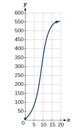
For the following exercises, use this scenario: The population \(P\) of an endangered species habitat for wolves is modeled by the function \(P(x) = \frac{558}{1 + 54.8e^{- 0.462x}},\) where \(x\) is given in years.
21. Graph the population model to show the population over a span of \(10\) years.
Solution (click to reveal)
22. What was the initial population of wolves transported to the habitat?
23. How many wolves will the habitat have after \(3\) years?
Solution (click to reveal)
About 38 wolves
24. How many years will it take before there are \(100\) wolves in the habitat?
25. Use the intersect feature to approximate the number of years it will take before the population of the habitat reaches half its carrying capacity.
Solution (click to reveal)
About 8.7 years
For the following exercises, refer to Table 7.
| \(x\) | 1 | 2 | 3 | 4 | 5 | 6 |
| f(x) | 1125 | 1495 | 2310 | 3294 | 4650 | 6361 |
Table 7
26. Use a graphing calculator to create a scatter diagram of the data.
27. Use the regression feature to find an exponential function that best fits the data in the table.
Solution (click to reveal)
\(f(x) = 776.682(1.426)^{x}\)
28. Write the exponential function as an exponential equation with base \(e.\)
29. Graph the exponential equation on the scatter diagram.
Solution (click to reveal)
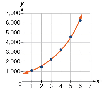
30. Use the intersect feature to find the value of \(x\) for which \(f(x) = 4000.\)
For the following exercises, refer to Table 8.
| \(x\) | 1 | 2 | 3 | 4 | 5 | 6 |
| f(x) | 555 | 383 | 307 | 210 | 158 | 122 |
Table 8
31. Use a graphing calculator to create a scatter diagram of the data.
Solution (click to reveal)
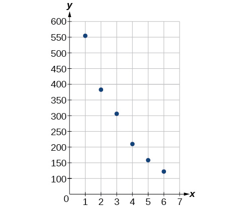
32. Use the regression feature to find an exponential function that best fits the data in the table.
33. Write the exponential function as an exponential equation with base \(e.\)
Solution (click to reveal)
\(f(x) = {731.92e}^{-0.3038x}\)
34. Graph the exponential equation on the scatter diagram.
35. Use the intersect feature to find the value of \(x\) for which \(f(x) = 250.\)
Solution (click to reveal)
When \(f(x) = 250,\operatorname{}x \approx 3.6\)
For the following exercises, refer to Table 9.
| \(x\) | 1 | 2 | 3 | 4 | 5 | 6 |
| f(x) | 5.1 | 6.3 | 7.3 | 7.7 | 8.1 | 8.6 |
Table 9
36. Use a graphing calculator to create a scatter diagram of the data.
37. Use the LOGarithm option of the REGression feature to find a logarithmic function of the form \(y = a + b\ln(x)\) that best fits the data in the table.
Solution (click to reveal)
\(y = 5.063 + 1.934\text{log}(x)\)
38. Use the logarithmic function to find the value of the function when \(x = 10.\)
39. Graph the logarithmic equation on the scatter diagram.
Solution (click to reveal)
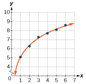
40. Use the intersect feature to find the value of \(x\) for which \(f(x) = 7.\)
For the following exercises, refer to Table 10.
| \(x\) | 1 | 2 | 3 | 4 | 5 | 6 | 7 | 8 |
| f(x) | 7.5 | 6 | 5.2 | 4.3 | 3.9 | 3.4 | 3.1 | 2.9 |
Table 10
41. Use a graphing calculator to create a scatter diagram of the data.
Solution (click to reveal)
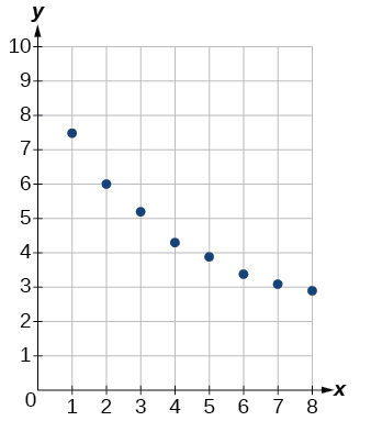
42. Use the LOGarithm option of the REGression feature to find a logarithmic function of the form \(y = a + b\ln(x)\) that best fits the data in the table.
43. Use the logarithmic function to find the value of the function when \(x = 10.\)
Solution (click to reveal)
When \(f(10) \approx 2.3\)
44. Graph the logarithmic equation on the scatter diagram.
45. Use the intersect feature to find the value of \(x\) for which \(f(x) = 8.\)
Solution (click to reveal)
When \(f(x) = 8,\operatorname{}x \approx 0.82\)
For the following exercises, refer to Table 11.
| \(x\) | 1 | 2 | 3 | 4 | 5 | 6 | 7 | 8 | 9 | 10 |
| f(x) | 8.7 | 12.3 | 15.4 | 18.5 | 20.7 | 22.5 | 23.3 | 24 | 24.6 | 24.8 |
Table 11
46. Use a graphing calculator to create a scatter diagram of the data.
47. Use the LOGISTIC regression option to find a logistic growth model of the form \(y = \frac{c}{1 + ae^{- bx}}\) that best fits the data in the table.
Solution (click to reveal)
\(f(x) = \frac{25.081}{1 + 3.182e^{- 0.545x}}\)
48. Graph the logistic equation on the scatter diagram.
49. To the nearest whole number, what is the predicted carrying capacity of the model?
Solution (click to reveal)
About 25
50. Use the intersect feature to find the value of \(x\) for which the model reaches half its carrying capacity.
For the following exercises, refer to Table 12.
| \(x\) | 0 | 2 | 4 | 5 | 7 | 8 | 10 | 11 | 15 | 17 |
| \(f(x)\) | 12 | 28.6 | 52.8 | 70.3 | 99.9 | 112.5 | 125.8 | 127.9 | 135.1 | 135.9 |
Table 12
51. Use a graphing calculator to create a scatter diagram of the data.
Solution (click to reveal)
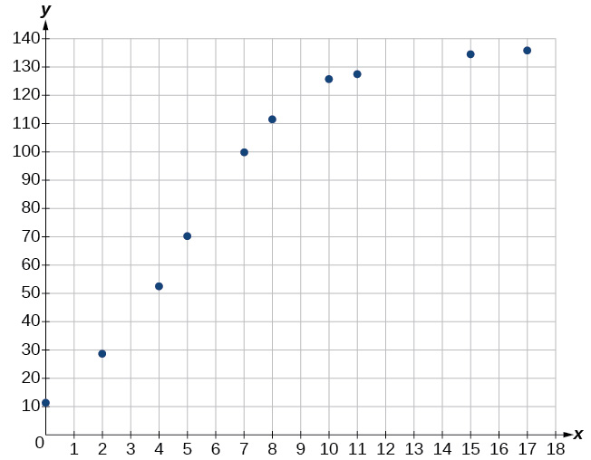
52. Use the LOGISTIC regression option to find a logistic growth model of the form \(y = \frac{c}{1 + ae^{- bx}}\) that best fits the data in the table.
53. Graph the logistic equation on the scatter diagram.
Solution (click to reveal)
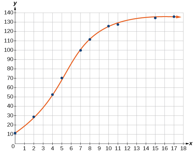
54. To the nearest whole number, what is the predicted carrying capacity of the model?
55. Use the intersect feature to find the value of \(x\) for which the model reaches half its carrying capacity.
Solution (click to reveal)
When \(f(x) = 68,\operatorname{}x \approx 4.9\)
Extensions
56. Recall that the general form of a logistic equation for a population is given by \(P(t) = \frac{c}{1 + ae^{- bt}},\) such that the initial population at time \(t = 0\) is \(P(0) = P_{0}.\) Show algebraically that \(\frac{c - P(t)}{P(t)} = \frac{c - P_{0}}{P_{0}}e^{- bt}.\)
57. Use a graphing utility to find an exponential regression formula \(f(x)\) and a logarithmic regression formula \(g(x)\) for the points \(\left( {1.5,1.5} \right)\) and \(\left( {8.5,\mspace{9mu}\text{8.5}} \right).\) Round all numbers to 6 decimal places. Graph the points and both formulas along with the line \(y = x\) on the same axis. Make a conjecture about the relationship of the regression formulas.
Solution (click to reveal)
\(f(x) = 1.034341(1.281204)^{x}\) ; \(g(x) = 4.035510\) ; the regression curves are symmetrical about \(y = x\) , so it appears that they are inverse functions.
58. Verify the conjecture made in the previous exercise. Round all numbers to six decimal places when necessary.
59. Find the inverse function \(f^{- 1}(x)\) for the logistic function \(f(x) = \frac{c}{1 + ae^{- bx}}.\) Show all steps.
Solution (click to reveal)
\({f^{- 1}(x)} = \frac{\text{ln}(a) - \text{ln}\left( \frac{c}{x} - 1 \right)}{b}\)
60. Use the result from the previous exercise to graph the logistic model \(P(t) = \frac{20}{1 + 4e^{- 0.5t}}\) along with its inverse on the same axis. What are the intercepts and asymptotes of each function?