5.6 Rational Functions
Suppose we know that the cost of making a product is dependent on the number of items, \(x,\) produced. This is given by the equation \(C(x) = 15{,}000x - 0.1x^{2} + 1000.\) If we want to know the average cost for producing \(x\) items, we would divide the cost function by the number of items, \(x.\)
The average cost function, which yields the average cost per item for \(x\) items produced, is
\[f(x) = \frac{15{,}000x - 0.1x^{2} + 1000}{x}\]
Many other application problems require finding an average value in a similar way, giving us variables in the denominator. Written without a variable in the denominator, this function will contain a negative integer power.
In the last few sections, we have worked with polynomial functions, which are functions with non-negative integers for exponents. In this section, we explore rational functions, which have variables in the denominator.
5.6.1 Using Arrow Notation
We have seen the graphs of the basic reciprocal function and the squared reciprocal function from our study of toolkit functions. Examine these graphs, as shown in Figure 1, and notice some of their features.
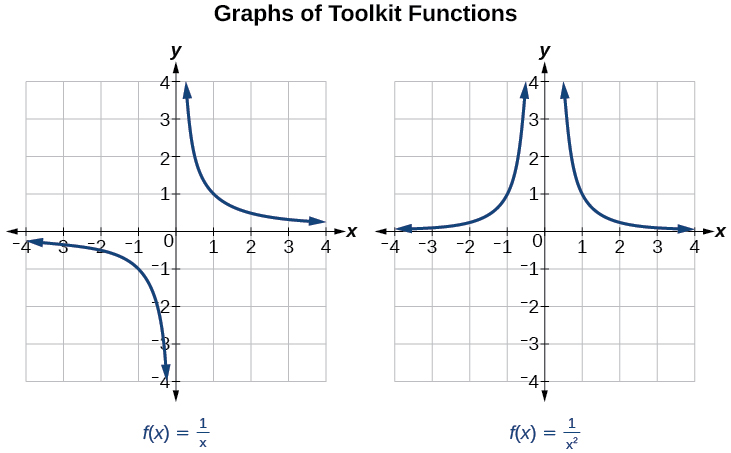
Figure 1
Several things are apparent if we examine the graph of \(f(x) = \frac{1}{x}.\)
- On the left branch of the graph, the curve approaches the \(x\)-axis \((y = 0)~\text{as}~x\rightarrow –\infty.\)
- As the graph approaches \(x = 0\) from the left, the curve drops, but as we approach zero from the right, the curve rises.
- Finally, on the right branch of the graph, the curves approaches the \(x\)-axis \((y = 0)~\text{as}~x\rightarrow\infty.\)
To summarize, we use arrow notation to show that \(x\) or \(f(x)\) is approaching a particular value. See Table 1.
| Symbol | Meaning |
|---|---|
| \(x\rightarrow a^{-}\) | \(x\) approaches \(a\) from the left ( \(x < a\) but close to \(a\) ) |
| \(x\rightarrow a^{+}\) | \(x\) approaches \(a\) from the right ( \(x > a\) but close to \(a\) ) |
| \(x\rightarrow\infty\) | \(x\) approaches infinity ( \(x\) increases without bound) |
| \(x\rightarrow - \infty\) | \(x\) approaches negative infinity ( \(x\) decreases without bound) |
| \(f(x)\rightarrow\infty\) | the output approaches infinity (the output increases without bound) |
| \(f(x)\rightarrow - \infty\) | the output approaches negative infinity (the output decreases without bound) |
| \(f(x)\rightarrow a\) | the output approaches \(a\) |
Table 1
Local Behavior of \(f(x) = \frac{1}{x}\)
Let’s begin by looking at the reciprocal function, \(f(x) = \frac{1}{x}.\) We cannot divide by zero, which means the function is undefined at \(x = 0;\) so zero is not in the domain. As the input values approach zero from the left side (becoming very small, negative values), the function values decrease without bound (in other words, they approach negative infinity). We can see this behavior in Table 2.
| \(x\) | –0.1 | –0.01 | –0.001 | –0.0001 |
| \(f(x) = \frac{1}{x}\) | –10 | –100 | –1000 | –10,000 |
Table 2
We write in arrow notation
\[\text{as~}x\rightarrow 0^{-},f(x)\rightarrow - \infty\]
As the input values approach zero from the right side (becoming very small, positive values), the function values increase without bound (approaching infinity). We can see this behavior in Table 3.
| \(x\) | 0.1 | 0.01 | 0.001 | 0.0001 |
| \(f(x) = \frac{1}{x}\) | 10 | 100 | 1000 | 10,000 |
Table 3
We write in arrow notation
\[\text{As~}x\rightarrow 0^{+},~f(x)\rightarrow\infty.\]
See Figure 2.
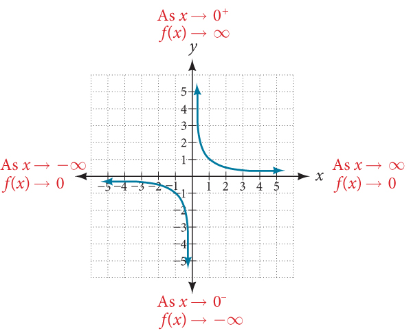
Figure 2
This behavior creates a vertical asymptote, which is a vertical line that the graph approaches but never crosses. In this case, the graph is approaching the vertical line \(x = 0\) as the input becomes close to zero. See Figure 3.
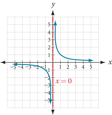
Figure 3
End Behavior of \(f(x) = \frac{1}{x}\)
As the values of \(x\) approach infinity, the function values approach 0. As the values of \(x\) approach negative infinity, the function values approach 0. See Figure 4. Symbolically, using arrow notation
\(\text{As~}x\rightarrow\infty,f(x)\rightarrow 0,\text{and~as~}x\rightarrow - \infty,f(x)\rightarrow 0.\)
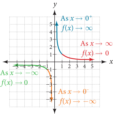
Figure 4
Based on this overall behavior and the graph, we can see that the function approaches 0 but never actually reaches 0; it seems to level off as the inputs become large. This behavior creates a horizontal asymptote, a horizontal line that the graph approaches as the input increases or decreases without bound. In this case, the graph is approaching the horizontal line \(y = 0.\) See Figure 5.
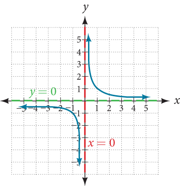
Figure 5
Use arrow notation to describe the end behavior and local behavior of the function graphed in Figure 6.
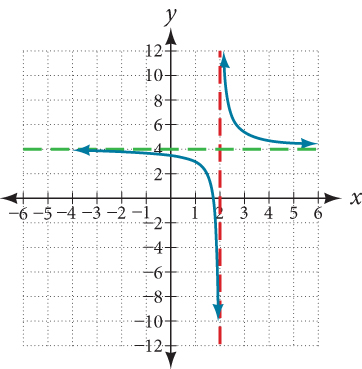
Figure 6
Solution (click to reveal)
Notice that the graph is showing a vertical asymptote at \(x = 2,\) which tells us that the function is undefined at \(x = 2.\)
\[\text{As~}x\rightarrow 2^{-},f(x)\rightarrow - \infty,\mspace{9mu}\text{and~as~}x\rightarrow 2^{+},\mspace{9mu} f(x)\rightarrow\infty.\]
And as the inputs decrease without bound, the graph appears to be leveling off at output values of 4, indicating a horizontal asymptote at \(y = 4.\) As the inputs increase without bound, the graph levels off at 4.
\[\text{As~}x\rightarrow\infty,\mspace{9mu} f(x)\rightarrow 4\mspace{9mu}\text{and~as~}x\rightarrow - \infty,\mspace{9mu} f(x)\rightarrow 4.\]
Sketch a graph of the reciprocal function shifted two units to the left and up three units. Identify the horizontal and vertical asymptotes of the graph, if any.
Solution (click to reveal)
Shifting the graph left 2 and up 3 would result in the function
\[f(x) = \frac{1}{x + 2} + 3\]
or equivalently, by giving the terms a common denominator,
\[f(x) = \frac{3x + 7}{x + 2}\]
The graph of the shifted function is displayed in Figure 7.
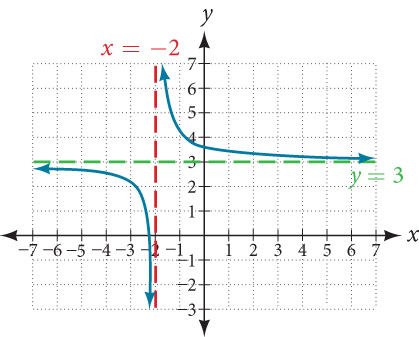
Figure 7
Notice that this function is undefined at \(x = -2,\) and the graph also is showing a vertical asymptote at \(x = -2.\)
\[\text{As~}x\rightarrow - 2^{-},~f(x)\rightarrow - \infty,\text{and~as}~x\rightarrow - 2^{+},~f(x)\rightarrow\infty.\]
As the inputs increase and decrease without bound, the graph appears to be leveling off at output values of 3, indicating a horizontal asymptote at \(y = 3.\)
\[\text{As~}x\rightarrow \pm \infty,~f(x)\rightarrow 3.\]
Notice that horizontal and vertical asymptotes are shifted left 2 and up 3 along with the function.
Sketch the graph, and find the horizontal and vertical asymptotes of the reciprocal squared function that has been shifted right 3 units and down 4 units.
Solution (click to reveal)
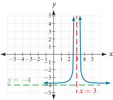
The function and the asymptotes are shifted 3 units right and 4 units down. As \(x\rightarrow 3,f(x)\rightarrow\infty,\) and as \(x\rightarrow \pm \infty,f(x)\rightarrow - 4.\)
The function is \(f(x) = \frac{1}{{(x - 3)}^{2}} - 4.\)
5.6.2 Solving Applied Problems Involving Rational Functions
In Example 2, we shifted a toolkit function in a way that resulted in the function \(f(x) = \frac{3x + 7}{x + 2}.\) This is an example of a rational function. A rational function is a function that can be written as the quotient of two polynomial functions. Many real-world problems require us to find the ratio of two polynomial functions. Problems involving rates and concentrations often involve rational functions.
5.6.3 Finding the Domains of Rational Functions
A vertical asymptote represents a value at which a rational function is undefined, so that value is not in the domain of the function. A reciprocal function cannot have values in its domain that cause the denominator to equal zero. In general, to find the domain of a rational function, we need to determine which inputs would cause division by zero.
Find the domain of \(f(x) = \frac{x + 3}{x^{2} - 9}.\)
Solution (click to reveal)
Begin by setting the denominator equal to zero and solving.
\[\begin{array}{rcl} {x^{2} - 9} & = & 0 \\ x^{2} & = & 9 \\ x & = & \pm 3 \end{array}\]
The denominator is equal to zero when \(x = \pm 3.\) The domain of the function is all real numbers except \(x = \pm 3.\)
A graph of this function, as shown in Figure 8, confirms that the function is not defined when \(x = \pm 3.\)
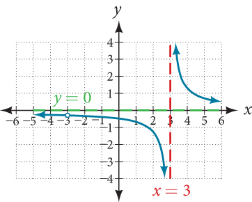
Figure 8
There is a vertical asymptote at \(x = 3\) and a hole in the graph at \(x = -3.\) We will discuss these types of holes in greater detail later in this section.
5.6.4 Identifying Vertical Asymptotes of Rational Functions
By looking at the graph of a rational function, we can investigate its local behavior and easily see whether there are asymptotes. We may even be able to approximate their location. Even without the graph, however, we can still determine whether a given rational function has any asymptotes, and calculate their location.
Vertical Asymptotes
The vertical asymptotes of a rational function may be found by examining the factors of the denominator that are not common to the factors in the numerator. Vertical asymptotes occur at the zeros of such factors.
Find the vertical asymptotes of the graph of \(k(x) = \frac{5 + 2x^{2}}{2 - x - x^{2}}.\)
Solution (click to reveal)
First, factor the numerator and denominator.
\[\begin{array}{ccl} {k(x)} & = & \frac{5 + 2x^{2}}{2 - x - x^{2}} \\ & = & \frac{5 + 2x^{2}}{(2 + x)(1 - x)} \end{array}\]
To find the vertical asymptotes, we determine where this function will be undefined by setting the denominator equal to zero:
\[\begin{array}{rcl} {(2 + x)(1 - x)} & = & 0 \\ x & = & {-2,1} \end{array}\]
Neither \(x = –2\) nor \(x = 1\) are zeros of the numerator, so the two values indicate two vertical asymptotes. The graph in Figure 9 confirms the location of the two vertical asymptotes.
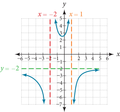
Figure 9
Removable Discontinuities
Occasionally, a graph will contain a hole: a single point where the graph is not defined, indicated by an open circle. We call such a hole a removable discontinuity.
For example, the function \(f(x) = \frac{x^{2} - 1}{x^{2} - 2x - 3}\) may be re-written by factoring the numerator and the denominator.
\[f(x) = \frac{\left( {x + 1} \right)\left( {x - 1} \right)}{\left( {x + 1} \right)\left( {x - 3} \right)}\]
Notice that \(x + 1\) is a common factor to the numerator and the denominator. The zero of this factor, \(x = -1,\) is the location of the removable discontinuity. Notice also that \(x–3\) is not a factor in both the numerator and denominator. The zero of this factor, \(x = 3,\) is the vertical asymptote. See Figure 10. [Note that removable discontinuities may not be visible when we use a graphing calculator, depending upon the window selected.]
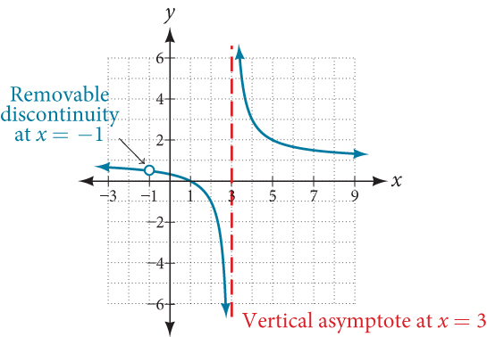
Figure 10
Find the vertical asymptotes and removable discontinuities of the graph of \(k(x) = \frac{x - 2}{x^{2} - 4}.\)
Solution (click to reveal)
Factor the numerator and the denominator.
\[k(x) = \frac{x - 2}{(x - 2)(x + 2)}\]
Notice that there is a common factor in the numerator and the denominator, \(x–2.\) The zero for this factor is \(x = 2.\) This is the location of the removable discontinuity.
Notice that there is a factor in the denominator that is not in the numerator, \(x + 2.\) The zero for this factor is \(x = -2.\) The vertical asymptote is \(x = -2.\) See Figure 11.
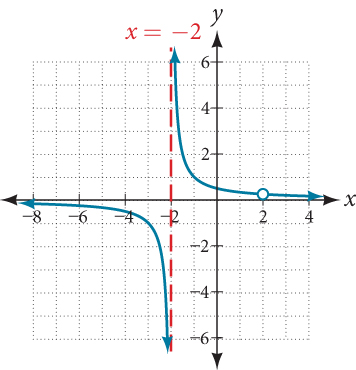
Figure 11
The graph of this function will have the vertical asymptote at \(x = -2,\) but at \(x = 2\) the graph will have a hole.
5.6.5 Identifying Horizontal Asymptotes of Rational Functions
While vertical asymptotes describe the behavior of a graph as the output gets very large or very small, horizontal asymptotes help describe the behavior of a graph as the input gets very large or very small. Recall that a polynomial’s end behavior will mirror that of the leading term. Likewise, a rational function’s end behavior will mirror that of the ratio of the function that is the ratio of the leading terms.
There are three distinct outcomes when checking for horizontal asymptotes:
Case 1: If the degree of the denominator > degree of the numerator, there is a horizontal asymptote at \(y = 0.\)
\[\text{Example:~}f(x) = \frac{4x + 2}{x^{2} + 4x - 5}\]
In this case, the end behavior is \(f(x) \approx \frac{4x}{x^{2}} = \frac{4}{x}.\) This tells us that, as the inputs increase or decrease without bound, this function will behave similarly to the function \(g(x) = \frac{4}{x},\) and the outputs will approach zero, resulting in a horizontal asymptote at \(y = 0.\) See Figure 12. Note that this graph crosses the horizontal asymptote.
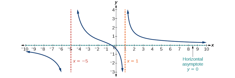
Figure 12 Horizontal asymptote \(y = 0\) when \(f(x) = \frac{p(x)}{q(x)},\mspace{9mu} q(x) \neq 0\mspace{9mu}\text{where~degree~of}\mspace{9mu} p < \text{degree~of~}q.\)
Case 2: If the degree of the denominator < degree of the numerator by one, we get a slant asymptote.
\[\text{Example:~}f(x) = \frac{3x^{2} - 2x + 1}{x - 1}\]
In this case, the end behavior is \(f(x) \approx \frac{3x^{2}}{x} = 3x.\) This tells us that as the inputs increase or decrease without bound, this function will behave similarly to the function \(g(x) = 3x.\) As the inputs grow large, the outputs will grow and not level off, so this graph has no horizontal asymptote. However, the graph of \(g(x) = 3x\) looks like a diagonal line, and since \(f\) will behave similarly to \(g,\) it will approach a line close to \(y = 3x.\) This line is a slant asymptote.
To find the equation of the slant asymptote, divide \(\frac{3x^{2} - 2x + 1}{x - 1}.\) The quotient is \(3x + 1,\) and the remainder is 2. The slant asymptote is the graph of the line \(g(x) = 3x + 1.\) See Figure 13.
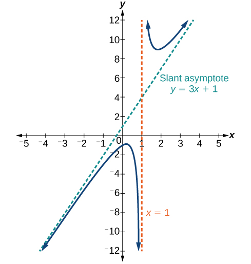
Figure 13 Slant asymptote when \(f(x) = \frac{p(x)}{q(x)},\mspace{9mu} q(x) \neq 0\) where degree of \(p > \text{degree~of~}q\mspace{9mu}\text{by}\mspace{9mu}\text{1}\text{.}\)
Case 3: If the degree of the denominator = degree of the numerator, there is a horizontal asymptote at \(y = \frac{a_{n}}{b_{n}},\) where \(a_{n}\) and \(b_{n}\) are the leading coefficients of \(p(x)\) and \(q(x)\) for \(f(x) = \frac{p(x)}{q(x)},q(x) \neq 0.\)
\[\text{Example:~}f(x) = \frac{3x^{2} + 2}{x^{2} + 4x - 5}\]
In this case, the end behavior is \(f(x) \approx \frac{3x^{2}}{x^{2}} = 3.\) This tells us that as the inputs grow large, this function will behave like the function \(g(x) = 3,\) which is a horizontal line. As \(x\rightarrow \pm \infty,f(x)\rightarrow 3,\) resulting in a horizontal asymptote at \(y = 3.\) See Figure 14. Note that this graph crosses the horizontal asymptote.
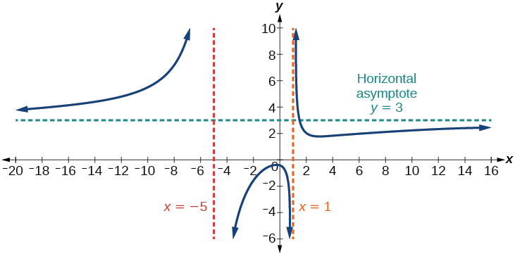
Figure 14 Horizontal asymptote when \(f(x) = \frac{p(x)}{q(x)},\mspace{9mu} q(x) \neq 0\mspace{9mu}\text{where~degree~of~}p = \text{degree~of~}q.\)
Notice that, while the graph of a rational function will never cross a vertical asymptote, the graph may or may not cross a horizontal or slant asymptote. Also, although the graph of a rational function may have many vertical asymptotes, the graph will have at most one horizontal (or slant) asymptote.
It should be noted that, if the degree of the numerator is larger than the degree of the denominator by more than one, the end behavior of the graph will mimic the behavior of the reduced end behavior fraction. For instance, if we had the function
\[f(x) = \frac{3x^{5} - x^{2}}{x + 3}\]
with end behavior
\[f(x) \approx \frac{3x^{5}}{x} = 3x^{4},\]
the end behavior of the graph would look similar to that of an even polynomial with a positive leading coefficient.
\[x\rightarrow \pm \infty,~f(x)\rightarrow\infty\]
For the functions listed, identify the horizontal or slant asymptote.
ⓐ \(g(x) = \frac{6x^{3} - 10x}{2x^{3} + 5x^{2}}\)
ⓑ \(h(x) = \frac{x^{2} - 4x + 1}{x + 2}\)
ⓒ \(k(x) = \frac{x^{2} + 4x}{x^{3} - 8}\)
Solution (click to reveal)
For these solutions, we will use \(f(x) = \frac{p(x)}{q(x)},~q(x) \neq 0.\)
ⓐ \(g(x) = \frac{6x^{3} - 10x}{2x^{3} + 5x^{2}}:\) The degree of \(p = \text{degree~of}~q = 3,\) so we can find the horizontal asymptote by taking the ratio of the leading terms. There is a horizontal asymptote at \(y = \frac{6}{2}\) or \(y = 3.\)
ⓑ \(h(x) = \frac{x^{2} - 4x + 1}{x + 2}:\) The degree of \(p = 2\) and degree of \(q = 1.\) Since \(p > q\) by 1, there is a slant asymptote found at \(\frac{x^{2} - 4x + 1}{x + 2}.\)

The quotient is \(x–6\) and the remainder is 13. There is a slant asymptote at \(y = x–6.\)
ⓒ \(k(x) = \frac{x^{2} + 4x}{x^{3} - 8}:\) The degree of \(p = 2\mspace{9mu} <\) degree of \(q = 3,\) so there is a horizontal asymptote \(y = 0.\)
Find the horizontal and vertical asymptotes of the function
\[f(x) = \frac{(x - 2)(x + 3)}{(x - 1)(x + 2)(x - 5)}\]
Solution (click to reveal)
First, note that this function has no common factors, so there are no potential removable discontinuities.
The function will have vertical asymptotes when the denominator is zero, causing the function to be undefined. The denominator will be zero at \(x = 1,–2,\text{and~}5,\) indicating vertical asymptotes at these values.
The numerator has degree 2, while the denominator has degree 3. Since the degree of the denominator is greater than the degree of the numerator, the denominator will grow faster than the numerator, causing the outputs to tend towards zero as the inputs get large, and so as \(x\rightarrow \pm \infty,~f(x)\rightarrow 0.\) This function will have a horizontal asymptote at \(y = 0.\) See Figure 15.
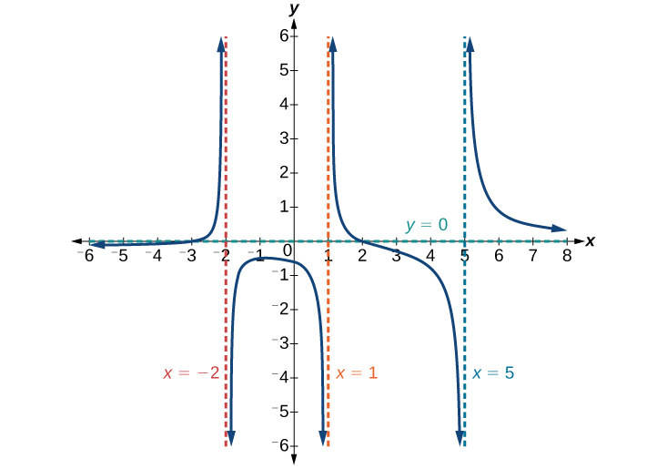
Figure 15
Find the intercepts of \(f(x) = \frac{(x - 2)(x + 3)}{(x - 1)(x + 2)(x - 5)}.\)
Solution (click to reveal)
We can find the \(y\)-intercept by evaluating the function at zero
\[\begin{array}{ccl} {f(0)} & = & \frac{(0 - 2)(0 + 3)}{(0 - 1)(0 + 2)(0 - 5)} \\ & = & \frac{- 6}{10} \\ & = & {- \frac{3}{5}} \\ & = & -0.6 \end{array}\]
The \(x\)-intercepts will occur when the function is equal to zero:
\[\begin{array}{rclc} 0 & = & \frac{(x - 2)(x + 3)}{(x - 1)(x + 2)(x - 5)} & {\qquad\text{This~is~zero~when~the~numerator~is~zero}.} \\ 0 & = & {(x - 2)(x + 3)} & \\ x & = & {2,-3} & \end{array}\]
The \(y\)-intercept is \((0,–0.6),\) the \(x\)-intercepts are \((2,0)\) and \((–3,0).\) See Figure 16.
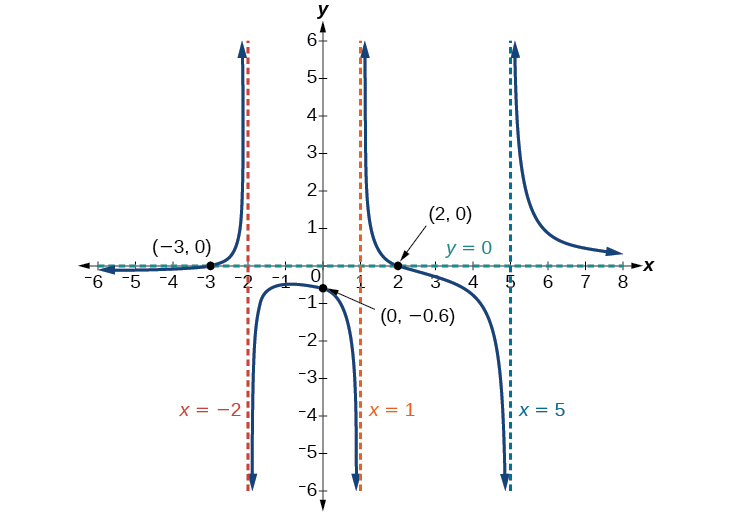
Figure 16
5.6.6 Graphing Rational Functions
In Example 9, we see that the numerator of a rational function reveals the \(x\)-intercepts of the graph, whereas the denominator reveals the vertical asymptotes of the graph. As with polynomials, factors of the numerator may have integer powers greater than one. Fortunately, the effect on the shape of the graph at those intercepts is the same as we saw with polynomials.
The vertical asymptotes associated with the factors of the denominator will mirror one of the two toolkit reciprocal functions. When the degree of the factor in the denominator is odd, the distinguishing characteristic is that on one side of the vertical asymptote the graph heads towards positive infinity, and on the other side the graph heads towards negative infinity. See Figure 17.
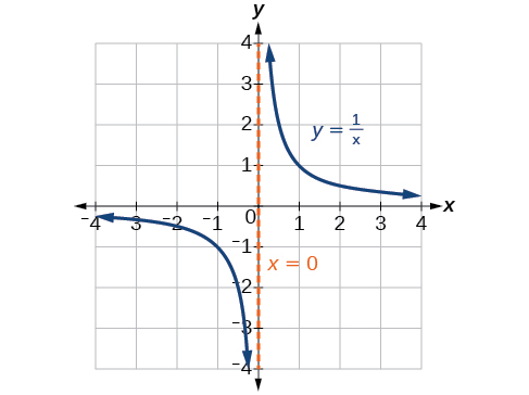
Figure 17
When the degree of the factor in the denominator is even, the distinguishing characteristic is that the graph either heads toward positive infinity on both sides of the vertical asymptote or heads toward negative infinity on both sides. See Figure 18.
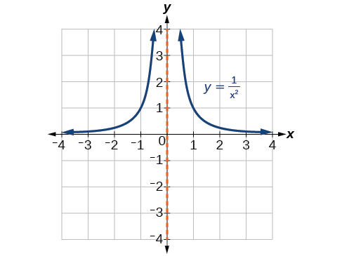
Figure 18
For example, the graph of \(f(x) = \frac{{(x + 1)}^{2}(x - 3)}{{(x + 3)}^{2}(x - 2)}\) is shown in Figure 19.
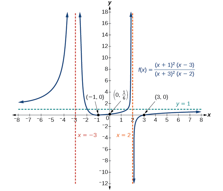
Figure 19
- At the \(x\)-intercept \(x = -1\) corresponding to the \({(x + 1)}^{2}\) factor of the numerator, the graph “bounces”, consistent with the quadratic nature of the factor.
- At the \(x\)-intercept \(x = 3\) corresponding to the \((x - 3)\) factor of the numerator, the graph passes through the axis as we would expect from a linear factor.
- At the vertical asymptote \(x = -3\) corresponding to the \({(x + 3)}^{2}\) factor of the denominator, the graph heads towards positive infinity on both sides of the asymptote, consistent with the behavior of the function \(f(x) = \frac{1}{x^{2}}.\)
- At the vertical asymptote \(x = 2,\) corresponding to the \((x - 2)\) factor of the denominator, the graph heads towards positive infinity on the left side of the asymptote and towards negative infinity on the right side.
Sketch a graph of \(f(x) = \frac{(x + 2)(x - 3)}{{(x + 1)}^{2}(x - 2)}.\)
Solution (click to reveal)
We can start by noting that the function is already factored, saving us a step.
Next, we will find the intercepts. Evaluating the function at zero gives the \(y\)-intercept:
\[\begin{array}{ccl} {f(0)} & = & \frac{(0 + 2)(0 - 3)}{{(0 + 1)}^{2}(0 - 2)} \\ & = & 3 \end{array}\]
To find the \(x\)-intercepts, we determine when the numerator of the function is zero. Setting each factor equal to zero, we find \(x\)-intercepts at \(x = –2\) and \(x = 3.\) At each, the behavior will be linear (multiplicity 1), with the graph passing through the intercept.
We have a \(y\)-intercept at \((0,3)\) and \(x\)-intercepts at \((–2,0)\) and \((3,0).\)
To find the vertical asymptotes, we determine when the denominator is equal to zero. This occurs when \(x + 1 = 0\) and when \(x–2 = 0,\) giving us vertical asymptotes at \(x = –1\) and \(x = 2.\)
There are no common factors in the numerator and denominator. This means there are no removable discontinuities.
Finally, the degree of denominator is larger than the degree of the numerator, telling us this graph has a horizontal asymptote at \(y = 0.\)
To sketch the graph, we might start by plotting the three intercepts. Since the graph has no \(x\)-intercepts between the vertical asymptotes, and the \(y\)-intercept is positive, we know the function must remain positive between the asymptotes, letting us fill in the middle portion of the graph as shown in Figure 20.
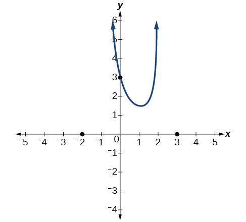
Figure 20
The factor associated with the vertical asymptote at \(x = -1\) was squared, so we know the behavior will be the same on both sides of the asymptote. The graph heads toward positive infinity as the inputs approach the asymptote on the right, so the graph will head toward positive infinity on the left as well.
For the vertical asymptote at \(x = 2,\) the factor was not squared, so the graph will have opposite behavior on either side of the asymptote. See Figure 21. After passing through the \(x\)-intercepts, the graph will then level off toward an output of zero, as indicated by the horizontal asymptote.
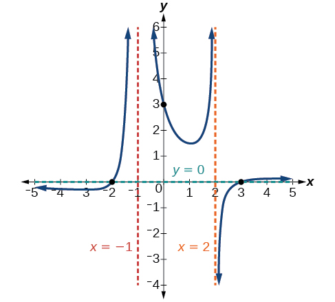
Figure 21
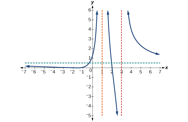
Given the function \(f(x) = \frac{{(x + 2)}^{2}(x - 2)}{2{(x - 1)}^{2}(x - 3)},\) use the characteristics of polynomials and rational functions to describe its behavior and sketch the function.
Solution (click to reveal)
Horizontal asymptote at \(y = \frac{1}{2}.\) Vertical asymptotes at \(x = 1~\text{and}~x = 3.\) \(y\)-intercept at \(\left( {0,\frac{4}{3}.} \right)\)
\(x\)-intercepts at \((2,0)~\mspace{9mu}\text{and~}(–2,0).\) \((–2,0)\) is a zero with multiplicity 2, and the graph bounces off the \(x\)-axis at this point. \((2,0)\) is a single zero and the graph crosses the axis at this point.
5.6.7 Writing Rational Functions
Now that we have analyzed the equations for rational functions and how they relate to a graph of the function, we can use information given by a graph to write the function. A rational function written in factored form will have an \(x\)-intercept where each factor of the numerator is equal to zero. (An exception occurs in the case of a removable discontinuity.) As a result, we can form a numerator of a function whose graph will pass through a set of \(x\)-intercepts by introducing a corresponding set of factors. Likewise, because the function will have a vertical asymptote where each factor of the denominator is equal to zero, we can form a denominator that will produce the vertical asymptotes by introducing a corresponding set of factors.
Write an equation for the rational function shown in Figure 22.
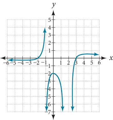
Figure 22
Solution (click to reveal)
The graph appears to have \(x\)-intercepts at \(x = –2\) and \(x = 3.\) At both, the graph passes through the intercept, suggesting linear factors. The graph has two vertical asymptotes. The one at \(x = –1\) seems to exhibit the basic behavior similar to \(\frac{1}{x},\) with the graph heading toward positive infinity on one side and heading toward negative infinity on the other. The asymptote at \(x = 2\) is exhibiting a behavior similar to \(\frac{1}{x^{2}},\) with the graph heading toward negative infinity on both sides of the asymptote. See Figure 23.
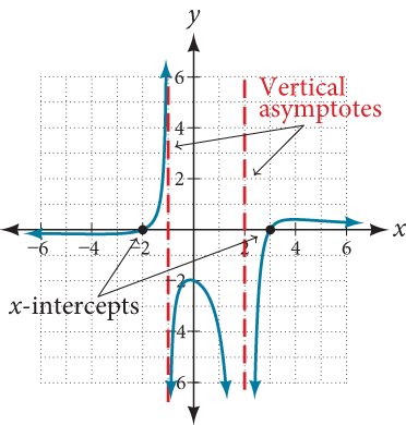
Figure 23
We can use this information to write a function of the form
\[f(x) = a\frac{(x + 2)(x - 3)}{(x + 1){(x - 2)}^{2}}\]
To find the stretch factor, we can use another clear point on the graph, such as the \(y\)-intercept \((0,–2).\)
\[\begin{array}{rcl} -2 & = & {a\frac{(0 + 2)(0 - 3)}{(0 + 1){(0 - 2)}^{2}}} \\ -2 & = & {a\frac{- 6}{4}} \\ a & = & {\frac{- 8}{- 6} = \frac{4}{3}} \end{array}\]
This gives us a final function of \(f(x) = \frac{4(x + 2)(x - 3)}{3(x + 1){(x - 2)}^{2}}.\)
Section Exercises
Verbal
1. What is the fundamental difference in the algebraic representation of a polynomial function and a rational function?
Solution (click to reveal)
The rational function will be represented by a quotient of polynomial functions.
2. What is the fundamental difference in the graphs of polynomial functions and rational functions?
3. If the graph of a rational function has a removable discontinuity, what must be true of the functional rule?
Solution (click to reveal)
The numerator and denominator must have a common factor.
4. Can a graph of a rational function have no vertical asymptote? If so, how?
5. Can a graph of a rational function have no \(x\)-intercepts? If so, how?
Solution (click to reveal)
Yes. The numerator of the formula of the functions would have only complex roots and/or factors common to both the numerator and denominator.
Algebraic
For the following exercises, find the domain of the rational functions.
6. \(f(x) = \frac{x - 1}{x + 2}\)
7. \(f(x) = \frac{x + 1}{x^{2} - 1}\)
Solution (click to reveal)
\(\text{All~reals~}x \neq –1,~1\)
8. \(f(x) = \frac{x^{2} + 4}{x^{2} - 2x - 8}\)
9. \(f(x) = \frac{x^{2} + 4x - 3}{x^{4} - 5x^{2} + 4}\)
Solution (click to reveal)
\(\text{All~reals~}x \neq –1,~–2,~1,~2\)
For the following exercises, find the domain, vertical asymptotes, and horizontal asymptotes of the functions.
10. \(f(x) = \frac{4}{x - 1}\)
11. \(f(x) = \frac{2}{5x + 2}\)
Solution (click to reveal)
V.A. at \(x = –\frac{2}{5};\) H.A. at \(y = 0;\) Domain is all reals \(x \neq –\frac{2}{5}\)
12. \(f(x) = \frac{x}{x^{2} - 9}\)
13. \(f(x) = \frac{x}{x^{2} + 5x - 36}\)
Solution (click to reveal)
V.A. at \(x = 4,~–9;\) H.A. at \(y = 0;\) Domain is all reals \(x \neq 4,~–9\)
14. \(f(x) = \frac{3 + x}{x^{3} - 27}\)
15. \(f(x) = \frac{3x - 4}{x^{3} - 16x}\)
Solution (click to reveal)
V.A. at \(x = 0,~4,~ - 4;\) H.A. at \(y = 0;\) Domain is all reals \(x \neq 0,4,~–4\)
16. \(f(x) = \frac{x^{2} - 1}{x^{3} + 9x^{2} + 14x}\)
17. \(f(x) = \frac{x + 5}{x^{2} - 25}\)
Solution (click to reveal)
V.A. at \(x = 5;\) H.A. at \(y = 0;\) Domain is all reals \(x \neq 5, - 5\)
18. \(f(x) = \frac{x - 4}{x - 6}\)
19. \(f(x) = \frac{4 - 2x}{3x - 1}\)
Solution (click to reveal)
V.A. at \(x = \frac{1}{3};\) H.A. at \(y = - \frac{2}{3};\) Domain is all reals \(x \neq \frac{1}{3}.\)
For the following exercises, find the \(x\)- and \(y\)-intercepts for the functions.
20. \(f(x) = \frac{x + 5}{x^{2} + 4}\)
21. \(f(x) = \frac{x}{x^{2} - x}\)
Solution (click to reveal)
none
22. \(f(x) = \frac{x^{2} + 8x + 7}{x^{2} + 11x + 30}\)
23. \(f(x) = \frac{x^{2} + x + 6}{x^{2} - 10x + 24}\)
Solution (click to reveal)
\(x\text{-intercepts~none,~}y\text{-intercept~}\left( {0,\frac{1}{4}} \right)\)
24. \(f(x) = \frac{94 - 2x^{2}}{3x^{2} - 12}\)
For the following exercises, describe the local and end behavior of the functions.
25. \(f(x) = \frac{x}{2x + 1}\)
Solution (click to reveal)
Local behavior: \(x\rightarrow - \frac{1}{2}^{+},f(x)\rightarrow - \infty,x\rightarrow - \frac{1}{2}^{-},f(x)\rightarrow\infty\)
End behavior: \(x\rightarrow \pm \infty,f(x)\rightarrow\frac{1}{2}\)
26. \(f(x) = \frac{2x}{x - 6}\)
27. \(f(x) = \frac{- 2x}{x - 6}\)
Solution (click to reveal)
Local behavior: \(x\rightarrow 6^{+},f(x)\rightarrow - \infty,x\rightarrow 6^{-},f(x)\rightarrow\infty,\) End behavior: \(x\rightarrow \pm \infty,f(x)\rightarrow - 2\)
28. \(f(x) = \frac{x^{2} - 4x + 3}{x^{2} - 4x - 5}\)
29. \(f(x) = \frac{2x^{2} - 32}{6x^{2} + 13x - 5}\)
Solution (click to reveal)
Local behavior: \(x\rightarrow\frac{1}{3}^{+},f(x)\rightarrow - \infty,x\rightarrow\frac{1}{3}^{-},\) \(f(x)\rightarrow\infty,x\rightarrow{- \frac{5}{2}}^{+},f(x)\rightarrow\infty,x\rightarrow{- \frac{5}{2}}^{–},f(x)\rightarrow - \infty\)
End behavior: \(x\rightarrow \pm \infty,\ f(x)\rightarrow\frac{1}{3}\)
For the following exercises, find the slant asymptote of the functions.
30. \(f(x) = \frac{24x^{2} + 6x}{2x + 1}\)
31. \(f(x) = \frac{4x^{2} - 10}{2x - 4}\)
Solution (click to reveal)
\(y = 2x + 4\)
32. \(f(x) = \frac{81x^{2} - 18}{3x - 2}\)
33. \(f(x) = \frac{6x^{3} - 5x}{3x^{2} + 4}\)
Solution (click to reveal)
\(y = 2x\)
34. \(f(x) = \frac{x^{2} + 5x + 4}{x - 1}\)
Graphical
For the following exercises, use the given transformation to graph the function. Note the vertical and horizontal asymptotes.
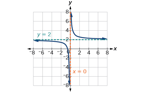
35. The reciprocal function shifted up two units.
Solution (click to reveal)
\(V.A.\mspace{9mu} x = 0,H.A.\mspace{9mu} y = 2\)
36. The reciprocal function shifted down one unit and left three units.
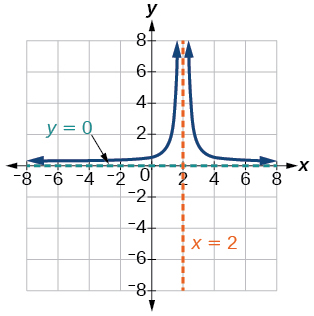
37. The reciprocal squared function shifted to the right 2 units.
Solution (click to reveal)
\(V.A.\mspace{9mu} x = 2,\mspace{9mu} H.A.\mspace{9mu} y = 0\)
38. The reciprocal squared function shifted down 2 units and right 1 unit.
For the following exercises, find the horizontal intercepts, the vertical intercept, the vertical asymptotes, and the horizontal or slant asymptote of the functions. Use that information to sketch a graph.
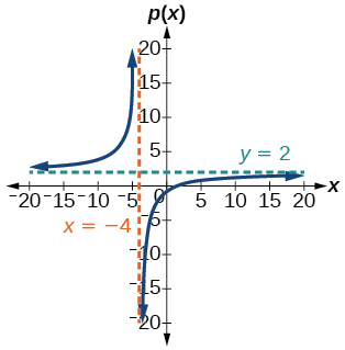
39. \(p(x) = \frac{2x - 3}{x + 4}\)
Solution (click to reveal)
\(V.A.\mspace{9mu} x = - 4,\mspace{9mu} H.A.\mspace{9mu} y = 2;\left( {\frac{3}{2},0} \right);\left( {0, - \frac{3}{4}} \right)\)
40. \(q(x) = \frac{x - 5}{3x - 1}\)
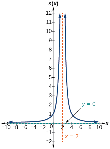
41. \(s(x) = \frac{4}{\left( {x - 2} \right)^{2}}\)
Solution (click to reveal)
\(V.A.\mspace{9mu} x = 2,\mspace{9mu} H.A.\mspace{9mu} y = 0,\mspace{9mu}(0,1)\)
42. \(r(x) = \frac{5}{\left( {x + 1} \right)^{2}}\)
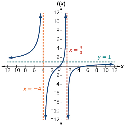
43. \(f(x) = \frac{3x^{2} - 14x - 5}{3x^{2} + 8x - 16}\)
Solution (click to reveal)
\(V.A.\mspace{9mu} x = - 4,\mspace{9mu} x = \frac{4}{3},\mspace{9mu} H.A.\mspace{9mu} y = 1;(5,0);\left( {- \frac{1}{3},0} \right);\left( {0,\frac{5}{16}} \right)\)
44. \(g(x) = \frac{2x^{2} + 7x - 15}{3x^{2} - 14x + 15}\)
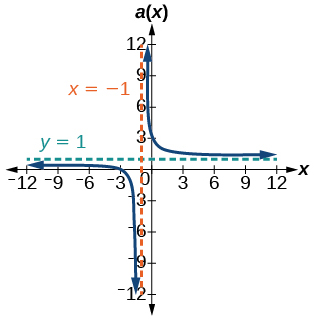
45. \(a(x) = \frac{x^{2} + 2x - 3}{x^{2} - 1}\)
Solution (click to reveal)
\(V.A.\mspace{9mu} x = - 1,\mspace{9mu} H.A.\mspace{9mu} y = 1;\left( {- 3,0} \right);\left( {0,3} \right)\)
46. \(b(x) = \frac{x^{2} - x - 6}{x^{2} - 4}\)
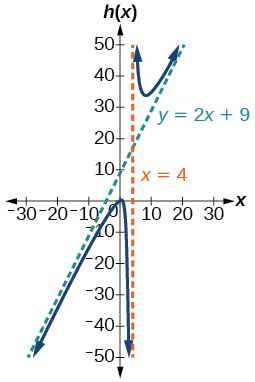
47. \(h(x) = \frac{2x^{2} + ~x - 1}{x - 4}\)
Solution (click to reveal)
\(V.A.\mspace{9mu} x = 4,\mspace{9mu} S.A.\mspace{9mu} y = 2x + 9;\left( {- 1,0} \right);\left( {\frac{1}{2},0} \right);\left( {0,\frac{1}{4}} \right)\)
48. \(k(x) = \frac{2x^{2} - 3x - 20}{x - 5}\)
49. \(w(x) = \frac{\left( {x - 1} \right)\left( {x + 3} \right)\left( {x - 5} \right)}{\left( {x + 2} \right)^{2}(x - 4)}\)
Solution (click to reveal)
\(V.A.\mspace{9mu} x = - 2,\mspace{9mu} x = 4,\mspace{9mu} H.A.\mspace{9mu} y = 1,\left( {1,0} \right);\left( {5,0} \right);\left( {- 3,0} \right);\left( {0, - \frac{15}{16}} \right)\)
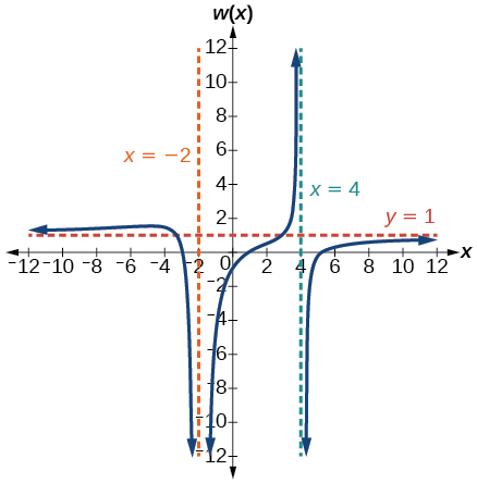
50. \(z(x) = \frac{\left( {x + 2} \right)^{2}\left( {x - 5} \right)}{\left( {x - 3} \right)\left( {x + 1} \right)\left( {x + 4} \right)}\)
For the following exercises, write an equation for a rational function with the given characteristics.
51. Vertical asymptotes at \(x = 5\) and \(x = -5,\) \(x\)-intercepts at \((2,0)\) and \((-1,0),\) \(y\)-intercept at \(\left( {0,4} \right)\)
Solution (click to reveal)
\(y = 50\frac{x^{2} - x - 2}{x^{2} - 25}\)
52. Vertical asymptotes at \(x = -4\) and \(x = -1,\) \(x\)-intercepts at \(\left( {1,0} \right)\) and \(\left( {5,0} \right),\) \(y\)-intercept at \((0,7)\)
53. Vertical asymptotes at \(x = -4\) and \(x = -5,\) \(x\)-intercepts at \(\left( {4,0} \right)\) and \(\left( {-6,0} \right),\) Horizontal asymptote at \(y = 7\)
Solution (click to reveal)
\(y = 7\frac{x^{2} + 2x - 24}{x^{2} + 9x + 20}\)
54. Vertical asymptotes at \(x = -3\) and \(x = 6,\) \(x\)-intercepts at \(\left( {-2,0} \right)\) and \(\left( {1,0} \right),\) Horizontal asymptote at \(y = -2\)
55. Vertical asymptote at \(x = -1,\) Double zero at \(x = 2,\) \(y\)-intercept at \((0,2)\)
Solution (click to reveal)
\(y = \frac{1}{2}\frac{x^{2} - 4x + 4}{x + 1}\)
56. Vertical asymptote at \(x = 3,\) Double zero at \(x = 1,\) \(y\)-intercept at \((0,4)\)
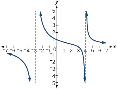
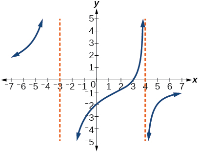
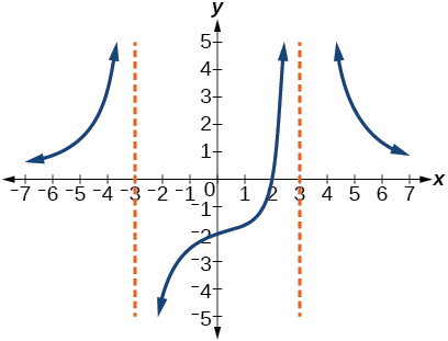
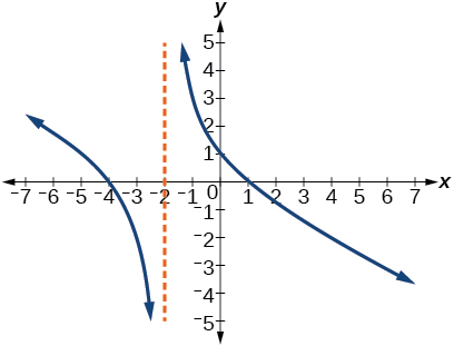
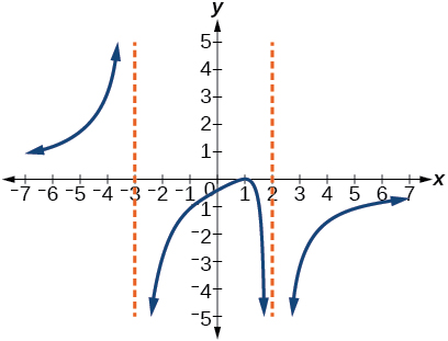
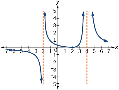
For the following exercises, use the graphs to write an equation for the function.
57.
Solution (click to reveal)
\(y = 4\frac{x - 3}{x^{2} - x - 12}\)
58.
59.
Solution (click to reveal)
\(y = \frac{27(x - 2)}{(x + 3)(x–3)^{2}}\)
60.
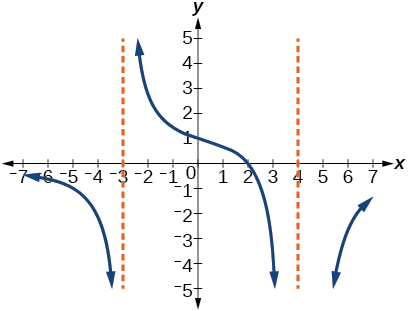
61.
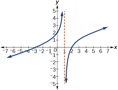
Solution (click to reveal)
\(y = \frac{1}{3}\frac{x^{2} + x - 6}{x - 1}\)
62.
63.
Solution (click to reveal)
\(y = - 6\frac{{(x - 1)}^{2}}{(x + 3){(x - 2)}^{2}}\)
64. Use \(\left( {0, - \frac{1}{2}} \right)\) as the additional point.
Numeric
For the following exercises, make tables to show the behavior of the function near the vertical asymptote and reflecting the horizontal asymptote
65. \(f(x) = \frac{1}{x - 2}\)
Solution (click to reveal)
| \(x\) | 2.01 | 2.001 | 2.0001 | 1.99 | 1.999 |
| \(y\) | 100 | 1,000 | 10,000 | –100 | –1,000 |
| \(x\) | 10 | 100 | 1,000 | 10,000 | 100,000 |
| \(y\) | .125 | .0102 | .001 | .0001 | .00001 |
Vertical asymptote \(x = 2,\) Horizontal asymptote \(y = 0\)
66. \(f(x) = \frac{x}{x - 3}\)
67. \(f(x) = \frac{2x}{x + 4}\)
Solution (click to reveal)
| \(x\) | –4.1 | –4.01 | –4.001 | –3.99 | –3.999 |
| \(y\) | 82 | 802 | 8,002 | –798 | –7998 |
| \(x\) | 10 | 100 | 1,000 | 10,000 | 100,000 |
| \(y\) | 1.4286 | 1.9331 | 1.992 | 1.9992 | 1.999992 |
Vertical asymptote \(x = - 4,\) Horizontal asymptote \(y = 2\)
68. \(f(x) = \frac{2x}{{(x - 3)}^{2}}\)
69. \(f(x) = \frac{x^{2}}{x^{2} + 2x + 1}\)
Solution (click to reveal)
| \(x\) | –.9 | –.99 | –.999 | –1.1 | –1.01 |
| \(y\) | 81 | 9,801 | 998,001 | 121 | 10,201 |
| \(x\) | 10 | 100 | 1,000 | 10,000 | 100,000 |
| \(y\) | .82645 | .9803 | .998 | .9998 |
Vertical asymptote \(x = - 1,\) Horizontal asymptote \(y = 1\)
Technology
For the following exercises, use a calculator to graph \(f(x).\) Use the graph to solve \(f(x) > 0.\)
70. \(f(x) = \frac{2}{x + 1}\)
71. \(f(x) = \frac{4}{2x - 3}\)
Solution (click to reveal)
\(\left( {\frac{3}{2},\infty} \right)\)
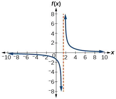
72. \(f(x) = \frac{2}{\left( {x - 1} \right)\left( {x + 2} \right)}\)
73. \(f(x) = \frac{x + 2}{\left( {x - 1} \right)\left( {x - 4} \right)}\)
Solution (click to reveal)
\(( - 2,1) \cup (4,\infty)\)
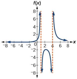
74. \(f(x) = \frac{{(x + 3)}^{2}}{\left( {x - 1} \right)^{2}\left( {x + 1} \right)}\)
Extensions
For the following exercises, identify the removable discontinuity.
75. \(f(x) = \frac{x^{2} - 4}{x - 2}\)
Solution (click to reveal)
\(\left( {2,4} \right)\)
76. \(f(x) = \frac{x^{3} + 1}{x + 1}\)
77. \(f(x) = \frac{x^{2} + x - 6}{x - 2}\)
Solution (click to reveal)
\(\left( {2,5} \right)\)
78. \(f(x) = \frac{2x^{2} + 5x - 3}{x + 3}\)
79. \(f(x) = \frac{x^{3} + x^{2}}{x + 1}\)
Solution (click to reveal)
\(\left( {–1,\text{1}} \right)\)
Real-World Applications
For the following exercises, express a rational function that describes the situation.
80. In the refugee camp hospital, a large mixing tank currently contains 200 gallons of water, into which 10 pounds of sugar have been mixed. A tap will open, pouring 10 gallons of water per minute into the tank at the same time sugar is poured into the tank at a rate of 3 pounds per minute. Find the concentration (pounds per gallon) of sugar in the tank after \(t\) minutes.
81. In the refugee camp hospital, a large mixing tank currently contains 300 gallons of water, into which 8 pounds of sugar have been mixed. A tap will open, pouring 20 gallons of water per minute into the tank at the same time sugar is poured into the tank at a rate of 2 pounds per minute. Find the concentration (pounds per gallon) of sugar in the tank after \(t\) minutes.
Solution (click to reveal)
\(C(t) = \frac{8 + 2t}{300 + 20t}\)
For the following exercises, use the given rational function to answer the question.
82. The concentration \(C\) of a drug in a patient’s bloodstream \(t\) hours after injection is given by \(C(t) = \frac{2t}{3 + t^{2}}.\) What happens to the concentration of the drug as \(t\) increases?
83. The concentration \(C\) of a drug in a patient’s bloodstream \(t\) hours after injection is given by \(C(t) = \frac{100t}{2t^{2} + 75}.\) Use a calculator to approximate the time when the concentration is highest.
Solution (click to reveal)
After about 6.12 hours.
For the following exercises, construct a rational function that will help solve the problem. Then, use a calculator to answer the question.
84. An open box with a square base is to have a volume of 108 cubic inches. Find the dimensions of the box that will have minimum surface area. Let \(x\) = length of the side of the base.
85. A rectangular box with a square base is to have a volume of 20 cubic feet. The material for the base costs 30 cents/ square foot. The material for the sides costs 10 cents/square foot. The material for the top costs 20 cents/square foot. Determine the dimensions that will yield minimum cost. Let \(x\) = length of the side of the base.
Solution (click to reveal)
\(A(x) = 50x^{2} + \frac{800}{x}.\) 2 by 2 by 5 feet.
86. A right circular cylinder has volume of 100 cubic inches. Find the radius and height that will yield minimum surface area. Let \(x\) = radius.
87. A right circular cylinder with no top has a volume of 50 cubic meters. Find the radius that will yield minimum surface area. Let \(x\) = radius.
Solution (click to reveal)
\(A(x) = \pi x^{2} + \frac{100}{x}.\) Radius = 2.52 meters.
88. A right circular cylinder is to have a volume of 40 cubic inches. It costs 4 cents/square inch to construct the top and bottom and 1 cent/square inch to construct the rest of the cylinder. Find the radius to yield minimum cost. Let \(x\) = radius.