4.1 Linear Functions
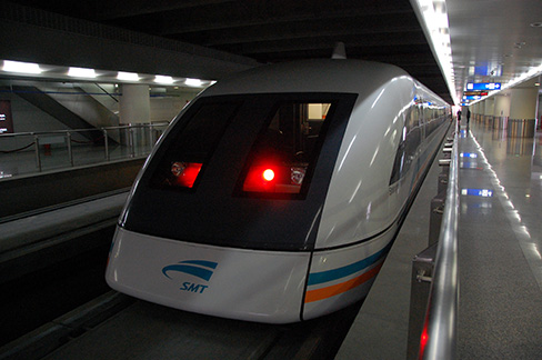
Figure 1 Shanghai MagLev Train (credit: “kanegen”/Flickr)
Just as with the growth of a bamboo plant, there are many situations that involve constant change over time. Consider, for example, the first commercial maglev train in the world, the Shanghai MagLev Train (Figure 1). It carries passengers comfortably for a 30-kilometer trip from the airport to the subway station in only eight minutes.
Suppose a maglev train travels a long distance, and maintains a constant speed of 83 meters per second for a period of time once it is 250 meters from the station. How can we analyze the train’s distance from the station as a function of time? In this section, we will investigate a kind of function that is useful for this purpose, and use it to investigate real-world situations such as the train’s distance from the station at a given point in time.
4.1.1 Representing Linear Functions
The function describing the train’s motion is a linear function, which is defined as a function with a constant rate of change. This is a polynomial of degree 1. There are several ways to represent a linear function, including word form, function notation, tabular form, and graphical form. We will describe the train’s motion as a function using each method.
Representing a Linear Function in Word Form
Let’s begin by describing the linear function in words. For the train problem we just considered, the following word sentence may be used to describe the function relationship.
- The train’s distance from the station is a function of the time during which the train moves at a constant speed plus its original distance from the station when it began moving at constant speed.
The speed is the rate of change. Recall that a rate of change is a measure of how quickly the dependent variable changes with respect to the independent variable. The rate of change for this example is constant, which means that it is the same for each input value. As the time (input) increases by 1 second, the corresponding distance (output) increases by 83 meters. The train began moving at this constant speed at a distance of 250 meters from the station.
Representing a Linear Function in Function Notation
Another approach to representing linear functions is by using function notation. One example of function notation is an equation written in the slope-intercept form of a line, where \(x\) is the input value, \(m\) is the rate of change, and \(b\) is the initial value of the dependent variable.
\[\begin{array}{ll} {\text{Equation~form}\qquad} & {y = mx + b} \\ {\text{Function~notation}\qquad} & {f(x) = mx + b} \end{array}\]
In the example of the train, we might use the notation \(D(t)\) where the total distance \(D\) is a function of the time \(t.\) The rate, \(m,\) is 83 meters per second. The initial value of the dependent variable \(b\) is the original distance from the station, 250 meters. We can write a generalized equation to represent the motion of the train.
\[D(t) = 83t + 250\]
Representing a Linear Function in Tabular Form
A third method of representing a linear function is through the use of a table. The relationship between the distance from the station and the time is represented in Figure 2. From the table, we can see that the distance changes by 83 meters for every 1 second increase in time.
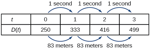
Figure 2 Tabular representation of the function \(D\) showing selected input and output values
Representing a Linear Function in Graphical Form
Another way to represent linear functions is visually, using a graph. We can use the function relationship from above, \(D(t) = 83t + 250,\) to draw a graph as represented in Figure 3. Notice the graph is a line. When we plot a linear function, the graph is always a line.
The rate of change, which is constant, determines the slant, or slope of the line. The point at which the input value is zero is the vertical intercept, or \(y\)-intercept, of the line. We can see from the graph that the \(y\)-intercept in the train example we just saw is \((0,250)\) and represents the distance of the train from the station when it began moving at a constant speed.
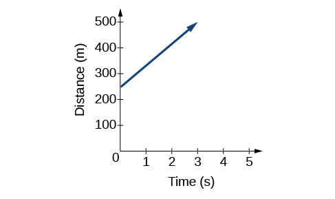
Figure 3 The graph of \(D(t) = 83t + 250\) . Graphs of linear functions are lines because the rate of change is constant.
Notice that the graph of the train example is restricted, but this is not always the case. Consider the graph of the line \(f(x) = 2x + 1.\) Ask yourself what numbers can be input to the function. In other words, what is the domain of the function? The domain is comprised of all real numbers because any number may be doubled, and then have one added to the product.
The pressure, \(P,\) in pounds per square inch (PSI) on the diver in Figure 4 depends upon her depth below the water surface, \(d,\) in feet. This relationship may be modeled by the equation, \(P(d) = 0.434d + 14.696.\) Restate this function in words.

Figure 4 (credit: Ilse Reijs and Jan-Noud Hutten)
Solution (click to reveal)
To restate the function in words, we need to describe each part of the equation. The pressure as a function of depth equals four hundred thirty-four thousandths times depth plus fourteen and six hundred ninety-six thousandths.
The initial value, 14.696, is the pressure in PSI on the diver at a depth of 0 feet, which is the surface of the water. The rate of change, or slope, is 0.434 PSI per foot. This tells us that the pressure on the diver increases 0.434 PSI for each foot her depth increases.
4.1.2 Determining Whether a Linear Function Is Increasing, Decreasing, or Constant
The linear functions we used in the two previous examples increased over time, but not every linear function does. A linear function may be increasing, decreasing, or constant. For an increasing function, as with the train example, the output values increase as the input values increase. The graph of an increasing function has a positive slope. A line with a positive slope slants upward from left to right as in Figure 5(a). For a decreasing function, the slope is negative. The output values decrease as the input values increase. A line with a negative slope slants downward from left to right as in Figure 5(b). If the function is constant, the output values are the same for all input values so the slope is zero. A line with a slope of zero is horizontal as in Figure 5(c).
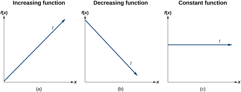
Figure 5
4.1.3 Interpreting Slope as a Rate of Change
In the examples we have seen so far, the slope was provided to us. However, we often need to calculate the slope given input and output values. Recall that given two values for the input, \(x_{1}\) and \(x_{2},\) and two corresponding values for the output, \(y_{1}\) and \(y_{2}\) —which can be represented by a set of points, \(\left( {x_{1}\text{,~}y_{1}} \right)\) and \(\left( {x_{2}\text{,~}y_{2}} \right)\) —we can calculate the slope \(m.\)
\[m = \frac{\text{change~in~output~(rise)}}{\text{change~in~input~(run)}} = \frac{\Delta y}{\Delta x} = \frac{y_{2} - y_{1}}{x_{2} - x_{1}}\]
Note that in function notation we can obtain two corresponding values for the output \(y_{1}\) and \(y_{2}\) for the function \(f,\) \(y_{1} = f\left( x_{1} \right)\) and \(y_{2} = f\left( x_{2} \right),\) so we could equivalently write
\[m = \frac{f\left( x_{2} \right)–f\left( x_{1} \right)}{x_{2}–x_{1}}\]
Figure 6 indicates how the slope of the line between the points, \(\left( {x_{1},y_{1}} \right)\) and \(\left( {x_{2},y_{2}} \right),\) is calculated. Recall that the slope measures steepness, or slant. The greater the absolute value of the slope, the steeper the slant is.
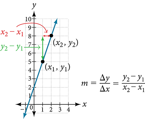
Figure 6 The slope of a function is calculated by the change in \(y\) divided by the change in \(x.\) It does not matter which coordinate is used as the \(\left( {x_{2,}y_{2}} \right)\) and which is the \(\left( {x_{1},y_{1}} \right),\) as long as each calculation is started with the elements from the same coordinate pair.
4.1.4 Writing and Interpreting an Equation for a Linear Function
Recall from Equations and Inequalities that we wrote equations in both the slope-intercept form and the point-slope form. Now we can choose which method to use to write equations for linear functions based on the information we are given. That information may be provided in the form of a graph, a point and a slope, two points, and so on. Look at the graph of the function \(f\) in Figure 7.
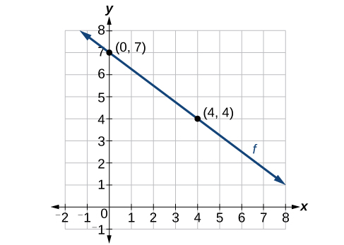
Figure 7
We are not given the slope of the line, but we can choose any two points on the line to find the slope. Let’s choose \((0,7)\) and \((4,4).\)
\[\begin{array}{ccl} m & = & \frac{y_{2} - y_{1}}{x_{2} - x_{1}} \\ & = & \frac{4 - 7}{4 - 0} \\ & = & {- \frac{3}{4}} \end{array}\]
Now we can substitute the slope and the coordinates of one of the points into the point-slope form.
\[\begin{array}{rcl} {y - y_{1}} & = & {m\left( x - x_{1} \right)} \\ {\mspace{9mu} y - 4} & = & {- \frac{3}{4}(x - 4)} \end{array}\]
If we want to rewrite the equation in the slope-intercept form, we would find
\[\begin{array}{rcl} {y - 4} & = & {- \frac{3}{4}(x - 4)} \\ {y - 4} & = & {- \frac{3}{4}x + 3} \\ y & = & {- \frac{3}{4}x + 7} \end{array}\]
If we want to find the slope-intercept form without first writing the point-slope form, we could have recognized that the line crosses the \(y\)-axis when the output value is 7. Therefore, \(b = 7.\) We now have the initial value \(b\) and the slope \(m\) so we can substitute \(m\) and \(b\) into the slope-intercept form of a line.

So the function is \(f(x) = - \frac{3}{4}x + 7,\) and the linear equation would be \(y = - \frac{3}{4}x + 7.\)
Write an equation for a linear function given a graph of \(f\) shown in Figure 8.
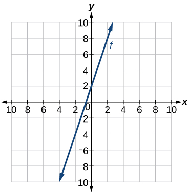
Figure 8
Solution (click to reveal)
Identify two points on the line, such as \((0,2)\) and \((-2,-4).\) Use the points to calculate the slope.
\[\begin{array}{ccl} m & = & \frac{y_{2} - y_{1}}{x_{2} - x_{1}} \\ & = & \frac{-4 - 2}{-2 - 0} \\ & = & \frac{-6}{-2} \\ & = & 3 \end{array}\]
Substitute the slope and the coordinates of one of the points into the point-slope form.
\[\begin{array}{rcl} {y - y_{1}} & = & {m\left( x - x_{1} \right)} \\ {y - (-4)} & = & {3(x - (-2))} \\ {y + 4} & = & {3(x + 2)} \end{array}\]
We can use algebra to rewrite the equation in the slope-intercept form.
\[\begin{array}{rcl} {y + 4} & = & {3(x + 2)} \\ {y + 4} & = & {3x + 6} \\ y & = & {3x + 2} \end{array}\]
This makes sense because we can see from Figure 9 that the line crosses the \(y\)-axis at the point \(\left( {0,\mspace{9mu} 2} \right),\) which is the \(y\)-intercept, so \(b = 2.\)
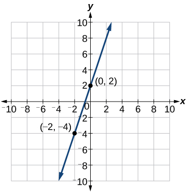
Figure 9
4.1.5 Modeling Real-World Problems with Linear Functions
In the real world, problems are not always explicitly stated in terms of a function or represented with a graph. Fortunately, we can analyze the problem by first representing it as a linear function and then interpreting the components of the function. As long as we know, or can figure out, the initial value and the rate of change of a linear function, we can solve many different kinds of real-world problems.
Marcus currently has 200 songs in his music collection. Every month, he adds 15 new songs. Write a formula for the number of songs, \(N,\) in his collection as a function of time, \(t,\) the number of months. How many songs will he own at the end of one year?
Solution (click to reveal)
The initial value for this function is 200 because he currently owns 200 songs, so \(N(0) = 200,\) which means that \(b = 200.\)
The number of songs increases by 15 songs per month, so the rate of change is 15 songs per month. Therefore we know that \(m = 15.\) We can substitute the initial value and the rate of change into the slope-intercept form of a line.

Figure 10
We can write the formula \(N(t) = 15t + 200.\)
With this formula, we can then predict how many songs Marcus will have at the end of one year (12 months). In other words, we can evaluate the function at \(t = 12.\)
\[\begin{array}{ccl} {N(12)} & = & {15(12) + 200} \\ & = & {180 + 200} \\ & = & 380 \end{array}\]
Marcus will have 380 songs in 12 months.
Notice that \(N\) is an increasing linear function. As the input (the number of months) increases, the output (number of songs) increases as well.
4.1.6 Graphing Linear Functions
Now that we’ve seen and interpreted graphs of linear functions, let’s take a look at how to create the graphs. There are three basic methods of graphing linear functions. The first is by plotting points and then drawing a line through the points. The second is by using the \(y\)-intercept and slope. And the third method is by using transformations of the identity function \(f(x) = x.\)
Graphing a Function by Plotting Points
To find points of a function, we can choose input values, evaluate the function at these input values, and calculate output values. The input values and corresponding output values form coordinate pairs. We then plot the coordinate pairs on a grid. In general, we should evaluate the function at a minimum of two inputs in order to find at least two points on the graph. For example, given the function, \(f(x) = 2x,\) we might use the input values 1 and 2. Evaluating the function for an input value of 1 yields an output value of 2, which is represented by the point \((1,2).\) Evaluating the function for an input value of 2 yields an output value of 4, which is represented by the point \((2,4).\) Choosing three points is often advisable because if all three points do not fall on the same line, we know we made an error.
Graph \(f(x) = - \frac{2}{3}x + 5\) by plotting points.
Solution (click to reveal)
Begin by choosing input values. This function includes a fraction with a denominator of 3, so let’s choose multiples of 3 as input values. We will choose 0, 3, and 6.
Evaluate the function at each input value, and use the output value to identify coordinate pairs.
\[\begin{aligned} {x = 0} & {\qquad f(0) = - \frac{2}{3}(0) + 5 = 5\Rightarrow(0,5)} \\ {x = 3} & {\qquad f(3) = - \frac{2}{3}(3) + 5 = 3\Rightarrow(3,3)} \\ {x = 6} & {\qquad f(6) = - \frac{2}{3}(6) + 5 = 1\Rightarrow(6,1)} \end{aligned}\]
Plot the coordinate pairs and draw a line through the points. Figure 11 represents the graph of the function \(f(x) = - \frac{2}{3}x + 5.\)
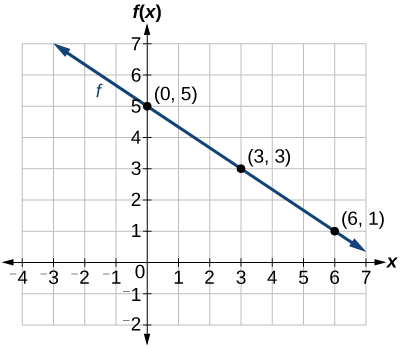
Figure 11 The graph of the linear function \(f(x) = - \frac{2}{3}x + 5.\)
The graph of the function is a line as expected for a linear function. In addition, the graph has a downward slant, which indicates a negative slope. This is also expected from the negative, constant rate of change in the equation for the function.
Graph \(f(x) = - \frac{3}{4}x + 6\) by plotting points.
Solution (click to reveal)
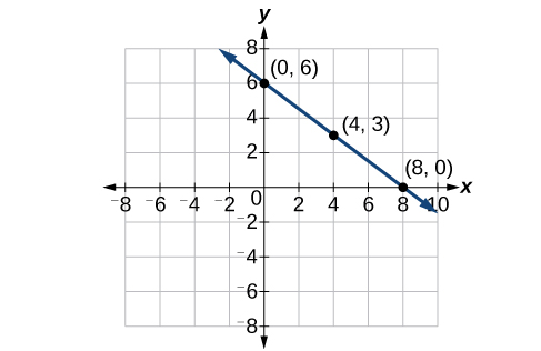
Graphing a Function Using \(y\)-intercept and Slope
Another way to graph linear functions is by using specific characteristics of the function rather than plotting points. The first characteristic is its \(y\)-intercept, which is the point at which the input value is zero. To find the \(y\)-intercept, we can set \(x = 0\) in the equation.
The other characteristic of the linear function is its slope.
Let’s consider the following function.
\[f(x) = \frac{1}{2}x + 1\]
The slope is \(\frac{1}{2}.\) Because the slope is positive, we know the graph will slant upward from left to right. The \(y\)-intercept is the point on the graph when \(x = 0.\) The graph crosses the \(y\)-axis at \((0,1).\) Now we know the slope and the \(y\)-intercept. We can begin graphing by plotting the point \((0,1).\) We know that the slope is the change in the \(y\)-coordinate over the change in the \(x\)-coordinate. This is commonly referred to as rise over run, \(m = \frac{\text{rise}}{\text{run}}.\) From our example, we have \(m = \frac{1}{2},\) which means that the rise is 1 and the run is 2. So starting from our \(y\)-intercept \((0,1),\) we can rise 1 and then run 2, or run 2 and then rise 1. We repeat until we have a few points, and then we draw a line through the points as shown in Figure 12.
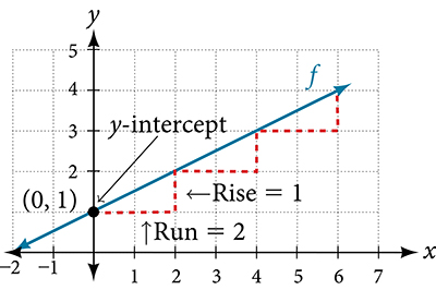
Figure 12
Graph \(f(x) = - \frac{2}{3}x + 5\) using the \(y\)-intercept and slope.
Solution (click to reveal)
Evaluate the function at \(x = 0\) to find the \(y\)-intercept. The output value when \(x = 0\) is 5, so the graph will cross the \(y\)-axis at \((0,5).\)
According to the equation for the function, the slope of the line is \(- \frac{2}{3}.\) This tells us that for each vertical decrease in the “rise” of \(–2\) units, the “run” increases by 3 units in the horizontal direction. We can now graph the function by first plotting the \(y\)-intercept on the graph in Figure 13. From the initial value \((0,5)\) we move down 2 units and to the right 3 units. We can extend the line to the left and right by repeating, and then drawing a line through the points.
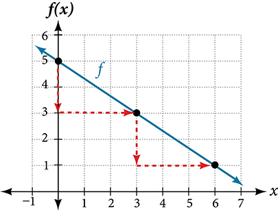
Figure 13 Graph of \(f(x) = -2/3x + 5\) and shows how to calculate the rise over run for the slope.
The graph slants downward from left to right, which means it has a negative slope as expected.
Graphing a Function Using Transformations
Another option for graphing is to use a transformation of the identity function \(f(x) = x.\) A function may be transformed by a shift up, down, left, or right. A function may also be transformed using a reflection, stretch, or compression.
Vertical Stretch or Compression
In the equation \(f(x) = mx,\) the \(m\) is acting as the vertical stretch or compression of the identity function. When \(m\) is negative, there is also a vertical reflection of the graph. Notice in Figure 14 that multiplying the equation of \(f(x) = x\) by \(m\) stretches the graph of \(f\) by a factor of \(m\) units if \(m > \text{1}\) and compresses the graph of \(f\) by a factor of \(m\) units if \(0 < m < 1.\) This means the larger the absolute value of \(m,\) the steeper the slope.
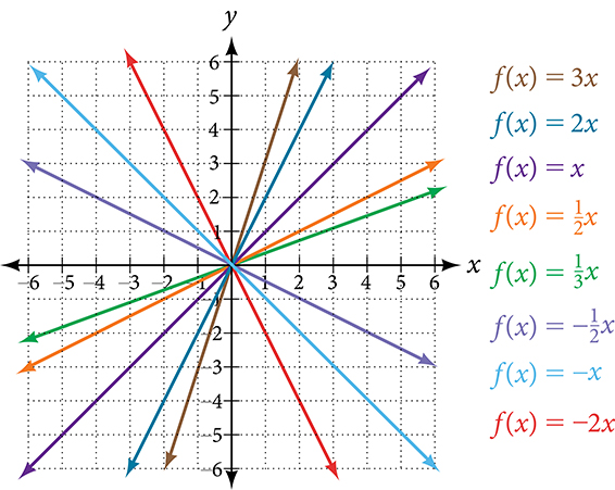
Figure 14 Vertical stretches and compressions and reflections on the function \(f(x) = x\)
Vertical Shift
In \(f(x) = mx + b,\) the \(b\) acts as the vertical shift, moving the graph up and down without affecting the slope of the line. Notice in Figure 15 that adding a value of \(b\) to the equation of \(f(x) = x\) shifts the graph of \(f\) a total of \(b\) units up if \(b\) is positive and \(|b|\) units down if \(b\) is negative.
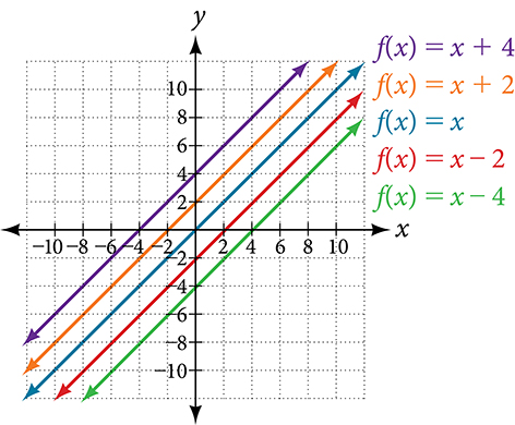
Figure 15 This graph illustrates vertical shifts of the function \(f(x) = x.\)
Using vertical stretches or compressions along with vertical shifts is another way to look at identifying different types of linear functions. Although this may not be the easiest way to graph this type of function, it is still important to practice each method.
Graph \(f(x) = \frac{1}{2}x - 3\) using transformations.
Solution (click to reveal)
The equation for the function shows that \(m = \frac{1}{2}\) so the identity function is vertically compressed by \(\frac{1}{2}.\) The equation for the function also shows that \(b = - 3\) so the identity function is vertically shifted down 3 units. First, graph the identity function, and show the vertical compression as in Figure 16.
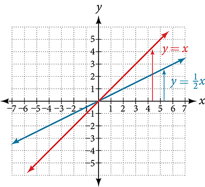
Figure 16 The function, \(y = x,\) compressed by a factor of \(\frac{1}{2}\) .
Then show the vertical shift as in Figure 17.
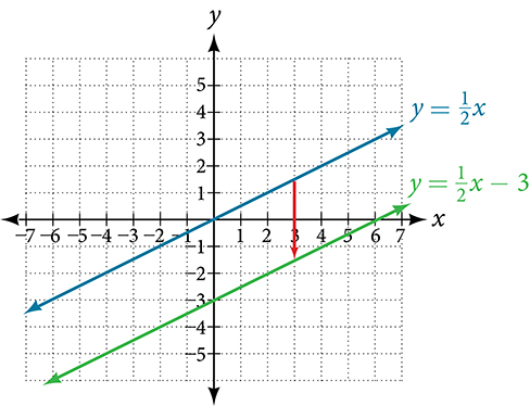
Figure 17 The function \(y = \frac{1}{2}x,\) shifted down 3 units.
Graph \(f(x) = 4 + 2x\) using transformations.
Solution (click to reveal)
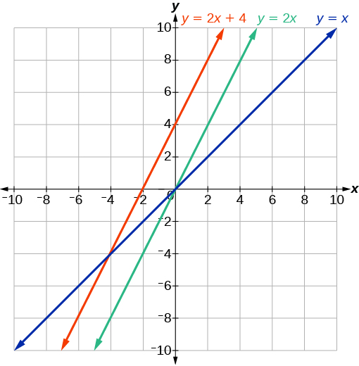
4.1.7 Writing the Equation for a Function from the Graph of a Line
Earlier, we wrote the equation for a linear function from a graph. Now we can extend what we know about graphing linear functions to analyze graphs a little more closely. Begin by taking a look at Figure 18. We can see right away that the graph crosses the \(y\)-axis at the point \((0,\text{4})\) so this is the \(y\)-intercept.
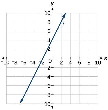
Figure 18
Then we can calculate the slope by finding the rise and run. We can choose any two points, but let’s look at the point \((–2,0).\) To get from this point to the \(y\)-intercept, we must move up 4 units (rise) and to the right 2 units (run). So the slope must be
\[m = \frac{\text{rise}}{\text{run}} = \frac{4}{2} = 2\]
Substituting the slope and \(y\)-intercept into the slope-intercept form of a line gives
\[y = 2x + 4\]
Match each equation of the linear functions with one of the lines in Figure 19.
ⓐ \(f(x) = 2x + 3\)
ⓑ \(g(x) = 2x - 3\)
ⓒ \(h(x) = - 2x + 3\)
ⓓ \(j(x) = \frac{1}{2}x + 3\)
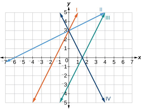
Figure 19
Solution (click to reveal)
Analyze the information for each function.
ⓐ This function has a slope of 2 and a \(y\)-intercept of 3. It must pass through the point (0, 3) and slant upward from left to right. We can use two points to find the slope, or we can compare it with the other functions listed. Function \(g\) has the same slope, but a different \(y\)-intercept. Lines I and III have the same slant because they have the same slope. Line III does not pass through \((0,\text{3})\) so \(f\) must be represented by line I.
ⓑ This function also has a slope of 2, but a \(y\)-intercept of \(-3.\) It must pass through the point \(\left( {0,-3} \right)\) and slant upward from left to right. It must be represented by line III.
ⓒ This function has a slope of –2 and a \(y\)-intercept of 3. This is the only function listed with a negative slope, so it must be represented by line IV because it slants downward from left to right.
ⓓ This function has a slope of \(\frac{1}{2}\) and a \(y\)-intercept of 3. It must pass through the point (0, 3) and slant upward from left to right. Lines I and II pass through \((0,\text{3}),\) but the slope of \(j\) is less than the slope of \(f\) so the line for \(j\) must be flatter. This function is represented by Line II.
Now we can re-label the lines as in Figure 20.
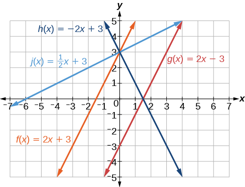
Figure 20
Finding the \(x\)-intercept of a Line
So far we have been finding the \(y\)-intercepts of a function: the point at which the graph of the function crosses the \(y\)-axis. Recall that a function may also have an \(x\)-intercept, which is the \(x\)-coordinate of the point where the graph of the function crosses the \(x\)-axis. In other words, it is the input value when the output value is zero.
To find the \(x\)-intercept, set a function \(f(x)\) equal to zero and solve for the value of \(x.\) For example, consider the function shown.
\[f(x) = 3x - 6\]
Set the function equal to 0 and solve for \(x.\)
\[\begin{array}{rcl} 0 & = & {3x - 6} \\ 6 & = & {3x} \\ 2 & = & x \\ x & = & 2 \end{array}\]
The graph of the function crosses the \(x\)-axis at the point \((2,\text{0}).\)
Do all linear functions have \(x\)-intercepts?
No. However, linear functions of the form \(y = c,\) where \(c\) is a nonzero real number are the only examples of linear functions with no x-intercept. For example, \(y = 5\) is a horizontal line 5 units above the x-axis. This function has no x-intercepts, as shown in Figure 21.
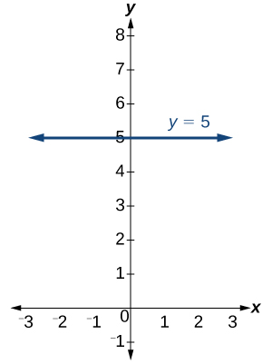
Figure 21
Find the \(x\)-intercept of \(f(x) = \frac{1}{2}x - 3.\)
Solution (click to reveal)
Set the function equal to zero to solve for \(x.\)
\[\begin{array}{rcl} 0 & = & {\frac{1}{2}x - 3} \\ 3 & = & {\frac{1}{2}x} \\ 6 & = & x \\ x & = & 6 \end{array}\]
The graph crosses the \(x\)-axis at the point \((6,\text{0}).\)
A graph of the function is shown in Figure 22. We can see that the \(x\)-intercept is \((6,\text{0})\) as we expected.
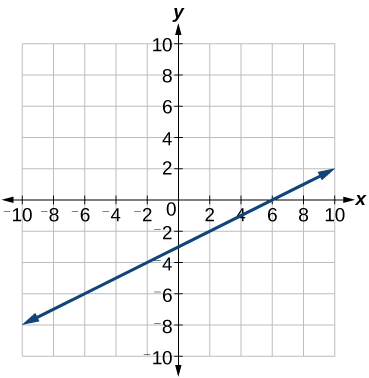
Figure 22
Describing Horizontal and Vertical Lines
There are two special cases of lines on a graph—horizontal and vertical lines. A horizontal line indicates a constant output, or \(y\)-value. In Figure 23, we see that the output has a value of 2 for every input value. The change in outputs between any two points, therefore, is 0. In the slope formula, the numerator is 0, so the slope is 0. If we use \(m = 0\) in the equation \(f(x) = mx + b,\) the equation simplifies to \(f(x) = b.\) In other words, the value of the function is a constant. This graph represents the function \(f(x) = 2.\)
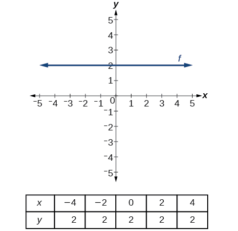
Figure 23 A horizontal line representing the function \(f(x) = 2\)
A vertical line indicates a constant input, or \(x\)-value. We can see that the input value for every point on the line is 2, but the output value varies. Because this input value is mapped to more than one output value, a vertical line does not represent a function. Notice that between any two points, the change in the input values is zero. In the slope formula, the denominator will be zero, so the slope of a vertical line is undefined.
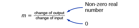
Figure 24 Example of how a line has a vertical slope. 0 in the denominator of the slope.
A vertical line, such as the one in Figure 25, has an \(x\)-intercept, but no \(y\)-intercept unless it’s the line \(x = 0.\) This graph represents the line \(x = 2.\)
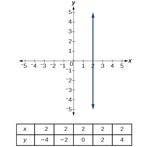
Figure 25 The vertical line, \(x = 2,\) which does not represent a function
Write the equation of the line graphed in Figure 26.
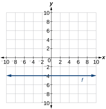
Figure 26
Solution (click to reveal)
For any \(x\)-value, the \(y\)-value is \(- 4,\) so the equation is \(y = - 4.\)
Write the equation of the line graphed in Figure 27.
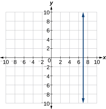
Figure 27
Solution (click to reveal)
The constant \(x\)-value is \(7,\) so the equation is \(x = 7.\)
4.1.8 Determining Whether Lines are Parallel or Perpendicular
The two lines in Figure 28 are parallel lines: they will never intersect. They have exactly the same steepness, which means their slopes are identical. The only difference between the two lines is the \(y\)-intercept. If we shifted one line vertically toward the other, they would become coincident.
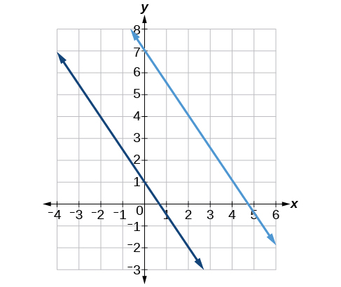
Figure 28 Parallel lines
We can determine from their equations whether two lines are parallel by comparing their slopes. If the slopes are the same and the \(y\)-intercepts are different, the lines are parallel. If the slopes are different, the lines are not parallel.
\[\begin{matrix} {\left. \begin{array}{l} {f(x) = - 2x + 6} \\ {f(x) = - 2x - 4} \end{array} \right\}\mspace{9mu}\text{parallel}\qquad} & {\left. \begin{array}{l} {f(x) = 3x + 2} \\ {f(x) = 2x + 2} \end{array} \right\}\mspace{9mu}\text{not~parallel}} \end{matrix}\]
Unlike parallel lines, perpendicular lines do intersect. Their intersection forms a right, or 90-degree, angle. The two lines in Figure 29 are perpendicular.
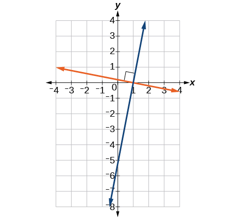
Figure 29 Perpendicular lines
Perpendicular lines do not have the same slope. The slopes of perpendicular lines are different from one another in a specific way. The slope of one line is the negative reciprocal of the slope of the other line. The product of a number and its reciprocal is \(1.\) So, if \(m_{1}\mspace{9mu}\text{and~}m_{2}\) are negative reciprocals of one another, they can be multiplied together to yield \(–1.\)
\[m_{1}m_{2} = -1\]
To find the reciprocal of a number, divide 1 by the number. So the reciprocal of 8 is \(\frac{1}{8},\) and the reciprocal of \(\frac{1}{8}\) is 8. To find the negative reciprocal, first find the reciprocal and then change the sign.
As with parallel lines, we can determine whether two lines are perpendicular by comparing their slopes, assuming that the lines are neither horizontal nor vertical. The slope of each line below is the negative reciprocal of the other so the lines are perpendicular.
\[\begin{array}{rcll} {f(x)} & = & {\frac{1}{4}x + 2} & {\qquad\text{negative~reciprocal~of}\mspace{9mu}\frac{1}{4}\mspace{9mu}\text{is~}-4} \\ {f(x)} & = & {-4x + 3} & {\qquad\text{negative~reciprocal~of}\mspace{9mu}-4\mspace{9mu}\text{is~}\frac{1}{4}} \end{array}\]
The product of the slopes is –1.
\[- 4\left( \frac{1}{4} \right) = - 1\]
Given the functions below, identify the functions whose graphs are a pair of parallel lines and a pair of perpendicular lines.
\[\begin{array}{rclrcl} {f(x)} & = & {2x + 3} & {\qquad h(x)} & = & {- 2x + 2} \\ {g(x)} & = & {\frac{1}{2}x - 4} & {\qquad j(x)} & = & {2x - 6} \end{array}\]
Solution (click to reveal)
Parallel lines have the same slope. Because the functions \(f(x) = 2x + 3\) and \(j(x) = 2x - 6\) each have a slope of 2, they represent parallel lines. Perpendicular lines have negative reciprocal slopes. Because −2 and \(\frac{1}{2}\) are negative reciprocals, the functions \(g(x) = \frac{1}{2}x - 4\) and \(h(x) = -2x + 2\) represent perpendicular lines.
A graph of the lines is shown in Figure 30.
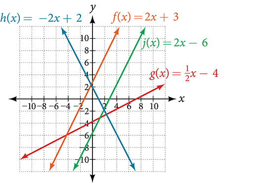
Figure 30
The graph shows that the lines \(f(x) = 2x + 3\) and \(j(x) = 2x–6\) are parallel, and the lines \(g(x) = \frac{1}{2}x–4\) and \(h(x) = - 2x + 2\) are perpendicular.
4.1.9 Writing the Equation of a Line Parallel or Perpendicular to a Given Line
If we know the equation of a line, we can use what we know about slope to write the equation of a line that is either parallel or perpendicular to the given line.
Writing Equations of Parallel Lines
Suppose for example, we are given the equation shown.
\[f(x) = 3x + 1\]
We know that the slope of the line formed by the function is 3. We also know that the \(y\)-intercept is \((0,1).\) Any other line with a slope of 3 will be parallel to \(f(x).\) So the lines formed by all of the following functions will be parallel to \(f(x).\)
\[\begin{array}{rcl} {g(x)} & = & {3x + 6} \\ {h(x)} & = & {3x + 1} \\ {p(x)} & = & {3x + \frac{2}{3}} \end{array}\]
Suppose then we want to write the equation of a line that is parallel to \(f\) and passes through the point \((1,\text{7}).\) This type of problem is often described as a point-slope problem because we have a point and a slope. In our example, we know that the slope is 3. We need to determine which value of \(b\) will give the correct line. We can begin with the point-slope form of an equation for a line, and then rewrite it in the slope-intercept form.
\[\begin{array}{rcl} {y - y_{1}} & = & {m\left( x - x_{1} \right)} \\ {y - 7} & = & {3(x - 1)} \\ {y - 7} & = & {3x - 3} \\ y & = & {3x + 4} \end{array}\]
So \(g(x) = 3x + 4\) is parallel to \(f(x) = 3x + 1\) and passes through the point \((1,\text{7}).\)
Find a line parallel to the graph of \(f(x) = 3x + 6\) that passes through the point \((3,\text{0}).\)
Solution (click to reveal)
The slope of the given line is 3. If we choose the slope-intercept form, we can substitute \(m = 3,x = 3,\) and \(f(x) = 0\) into the slope-intercept form to find the \(y\)-intercept.
\[\begin{array}{rcl} {g(x)} & = & {3x + b} \\ 0 & = & {3(3) + b} \\ b & = & –9 \end{array}\]
The line parallel to \(f(x)\) that passes through \((3,\text{0})\) is \(g(x) = 3x - 9.\)
We can confirm that the two lines are parallel by graphing them. Figure 31 shows that the two lines will never intersect.
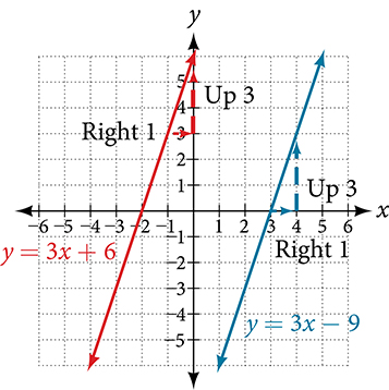
Figure 31
Writing Equations of Perpendicular Lines
We can use a very similar process to write the equation for a line perpendicular to a given line. Instead of using the same slope, however, we use the negative reciprocal of the given slope. Suppose we are given the function shown.
\[f(x) = 2x + 4\]
The slope of the line is 2, and its negative reciprocal is \(- \frac{1}{2}.\) Any function with a slope of \(- \frac{1}{2}\) will be perpendicular to \(f(x).\) So the lines formed by all of the following functions will be perpendicular to \(f(x).\)
\[\begin{array}{rcl} {g(x)} & = & {- \frac{1}{2}x + 4} \\ {h(x)} & = & {- \frac{1}{2}x + 2} \\ {p(x)} & = & {- \frac{1}{2}x - \frac{1}{2}} \end{array}\]
As before, we can narrow down our choices for a particular perpendicular line if we know that it passes through a given point. Suppose then we want to write the equation of a line that is perpendicular to \(f(x)\) and passes through the point \((4,\text{0}).\) We already know that the slope is \(- \frac{1}{2}.\) Now we can use the point to find the \(y\)-intercept by substituting the given values into the slope-intercept form of a line and solving for \(b.\)
\[\begin{array}{rcl} {g(x)} & = & {mx + b} \\ 0 & = & {- \frac{1}{2}(4) + b} \\ 0 & = & {-2 + b} \\ 2 & = & b \\ b & = & 2 \end{array}\]
The equation for the function with a slope of \(- \frac{1}{2}\) and a \(y\)-intercept of 2 is
\[g(x) = - \frac{1}{2}x + 2\]
So \(g(x) = - \frac{1}{2}x + 2\) is perpendicular to \(f(x) = 2x + 4\) and passes through the point \((4,\text{0}).\) Be aware that perpendicular lines may not look obviously perpendicular on a graphing calculator unless we use the square zoom feature.
Find the equation of a line perpendicular to \(f(x) = 3x + 3\) that passes through the point \((3,\text{0}).\)
Solution (click to reveal)
The original line has slope \(m = 3,\) so the slope of the perpendicular line will be its negative reciprocal, or \(- \frac{1}{3}.\) Using this slope and the given point, we can find the equation of the line.
\[\begin{array}{rcl} {g(x)} & = & {–\frac{1}{3}x + b} \\ 0 & = & {–\frac{1}{3}(3) + b} \\ 1 & = & b \\ b & = & 1 \end{array}\]
The line perpendicular to \(f(x)\) that passes through \((3,\text{0})\) is \(g(x) = - \frac{1}{3}x + 1.\)
A graph of the two lines is shown in Figure 32.
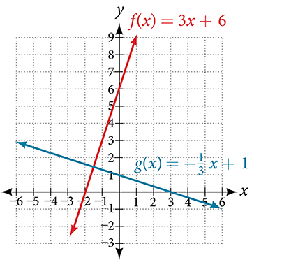
Figure 32
Note that that if we graph perpendicular lines on a graphing calculator using standard zoom, the lines may not appear to be perpendicular. Adjusting the window will make it possible to zoom in further to see the intersection more closely.
Section Exercises
Verbal
1. Terry is skiing down a steep hill. Terry’s elevation, \(E(t),\) in feet after \(t\) seconds is given by \(E(t) = 3000 - 70t.\) Write a complete sentence describing Terry’s starting elevation and how it is changing over time.
Solution (click to reveal)
Terry starts at an elevation of 3000 feet and descends 70 feet per second.
2. Jessica is walking home from a friend’s house. After 2 minutes she is 1.4 miles from home. Twelve minutes after leaving, she is 0.9 miles from home. What is her rate in miles per hour?
3. A boat is 100 miles away from the marina, sailing directly toward it at 10 miles per hour. Write an equation for the distance of the boat from the marina after \(t\) hours.
Solution (click to reveal)
\(d(t) = 100 - 10t\)
4. If the graphs of two linear functions are perpendicular, describe the relationship between the slopes and the \(y\)-intercepts.
5. If a horizontal line has the equation \(f(x) = a\) and a vertical line has the equation \(x = a,\) what is the point of intersection? Explain why what you found is the point of intersection.
Solution (click to reveal)
The point of intersection is \(\left( {a,\mspace{9mu} a} \right).\) This is because for the horizontal line, all of the \(y\) coordinates are \(a\) and for the vertical line, all of the \(x\) coordinates are \(a.\) The point of intersection is on both lines and therefore will have these two characteristics.
Algebraic
For the following exercises, determine whether the equation of the curve can be written as a linear function.
6. \(y = \frac{1}{4}x + 6\)
7. \(y = 3x - 5\)
Solution (click to reveal)
Yes
8. \(y = 3x^{2} - 2\)
9. \(3x + 5y = 15\)
Solution (click to reveal)
Yes
10. \(3x^{2} + 5y = 15\)
11. \(3x + 5y^{2} = 15\)
Solution (click to reveal)
No
12. \(- 2x^{2} + 3y^{2} = 6\)
13. \(- \frac{x - 3}{5} = 2y\)
Solution (click to reveal)
Yes
For the following exercises, determine whether each function is increasing or decreasing.
14. \(f(x) = 4x + 3\)
15. \(g(x) = 5x + 6\)
Solution (click to reveal)
Increasing
16. \(a(x) = 5 - 2x\)
17. \(b(x) = 8 - 3x\)
Solution (click to reveal)
Decreasing
18. \(h(x) = -2x + 4\)
19. \(k(x) = -4x + 1\)
Solution (click to reveal)
Decreasing
20. \(j(x) = \frac{1}{2}x - 3\)
21. \(p(x) = \frac{1}{4}x - 5\)
Solution (click to reveal)
Increasing
22. \(n(x) = - \frac{1}{3}x - 2\)
23. \(m(x) = - \frac{3}{8}x + 3\)
Solution (click to reveal)
Decreasing
For the following exercises, find the slope of the line that passes through the two given points.
24. \((2,4)\) and \((4,\text{10})\)
25. \((1,\text{5})\) and \((4,\text{11})\)
Solution (click to reveal)
2
26. \((–1,\text{4})\) and \((5,\text{2})\)
27. \((8,–2)\) and \((4,6)\)
Solution (click to reveal)
–2
28. \((6,11)\) and \((–4,\text{3})\)
For the following exercises, given each set of information, find a linear equation satisfying the conditions, if possible.
29. \(f( - 5) = -4,\) and \(f(5) = 2\)
Solution (click to reveal)
\(y = \frac{3}{5}x - 1\)
30. \(f(-1) = 4,\) and \(f(5) = 1\)
31. Passes through \((2,4)\) and \((4,10)\)
Solution (click to reveal)
\(y = 3x - 2\)
32. Passes through \((1,5)\) and \((4,11)\)
33. Passes through \((-1,\text{4})\) and \((5,2)\)
Solution (click to reveal)
\(y = - \frac{1}{3}x + \frac{11}{3}\)
34. Passes through \((-2,\text{8})\) and \((4,\text{6})\)
35. \(x\) intercept at \((-2,0)\) and \(y\) intercept at \((0,-3)\)
Solution (click to reveal)
\(y = - 1.5x - 3\)
36. \(x\) intercept at \((-5,\text{0})\) and \(y\) intercept at \((0,4)\)
For the following exercises, determine whether the lines given by the equations below are parallel, perpendicular, or neither.
37. \(\begin{array}{l} {4x - 7y = 10} \\ {7x + 4y = 1} \end{array}\)
Solution (click to reveal)
perpendicular
38. \(\begin{matrix} {3y + x = 12} \\ {- y = 8x + 1} \end{matrix}\)
39. \(\begin{matrix} {3y + 4x = 12} \\ {- 6y = 8x + 1} \end{matrix}\)
Solution (click to reveal)
parallel
40. \(\begin{array}{l} {6x - 9y = 10} \\ {3x + 2y = 1} \end{array}\)
For the following exercises, find the \(x\)- and \(y\)-intercepts of each equation.
41. \(f(x) = - x + 2\)
Solution (click to reveal)
\(\begin{array}{l} {f(0) = - (0) + 2} \\ {f(0) = 2} \\ {y - {int}:(0,2)} \\ {0 = - x + 2} \\ {x - {int}:(2,0)} \end{array}\)
42. \(g(x) = 2x + 4\)
43. \(h(x) = 3x - 5\)
Solution (click to reveal)
\(\begin{array}{l} {h(0) = 3(0) - 5} \\ {h(0) = - 5} \\ {y - {int}:(0, - 5)} \\ {0 = 3x - 5} \\ {x - {int}:\left( {\frac{5}{3},0} \right)} \end{array}\)
44. \(k(x) = -5x + 1\)
45. \(- 2x + 5y = 20\)
Solution (click to reveal)
\(\begin{array}{l} {- 2x + 5y = 20} \\ {- 2(0) + 5y = 20} \\ {5y = 20} \\ {y = 4} \\ {y - {int}:(0,4)} \\ {- 2x + 5(0) = 20} \\ {x = - 10} \\ {x - {int}:( - 10,0)} \end{array}\)
46. \(7x + 2y = 56\)
For the following exercises, use the descriptions of each pair of lines given below to find the slopes of Line 1 and Line 2. Is each pair of lines parallel, perpendicular, or neither?
47. Line 1: Passes through \((0,6)\) and \((3,-24)\)
Line 2: Passes through \((-1,19)\) and \((8,-71)\)
Solution (click to reveal)
Line 1: \(m\) = –10 Line 2: \(m\) = –10 Parallel
48. Line 1: Passes through \((-8,-55)\) and \((10,89)\)
Line 2: Passes through \((9, - 44)\) and \((4, - 14)\)
49. Line 1: Passes through \((2,3)\) and \((4,-1)\)
Line 2: Passes through \((6,3)\) and \((8,5)\)
Solution (click to reveal)
Line 1: \(m\) = –2 Line 2: \(m\) = 1 Neither
50. Line 1: Passes through \((1,7)\) and \((5,5)\)
Line 2: Passes through \((-1,-3)\) and \((1,1)\)
51. Line 1: Passes through \((2,5)\) and \((5, - 1)\)
Line 2: Passes through \((-3,7)\) and \((3,-5)\)
Solution (click to reveal)
\(\text{Line~1}:~m = –2~~~\text{Line~2}:~m = –2~~~\text{Parallel}\)
For the following exercises, write an equation for the line described.
52. Write an equation for a line parallel to \(f(x) = - 5x - 3\) and passing through the point \((2,\text{–}12).\)
53. Write an equation for a line parallel to \(g(x) = 3x - 1\) and passing through the point \((4,9).\)
Solution (click to reveal)
\(y = 3x - 3\)
54. Write an equation for a line perpendicular to \(h(t) = -2t + 4\) and passing through the point \((-4,–1).\)
55. Write an equation for a line perpendicular to \(p(t) = 3t + 4\) and passing through the point \((3,1).\)
Solution (click to reveal)
\(y = - \frac{1}{3}t + 2\)
Graphical
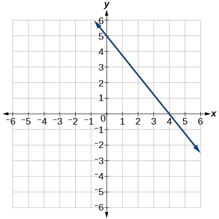
For the following exercises, find the slope of the line graphed.
56.
57.
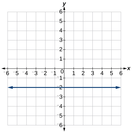
Solution (click to reveal)
0
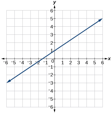
For the following exercises, write an equation for the line graphed.
58.
59.
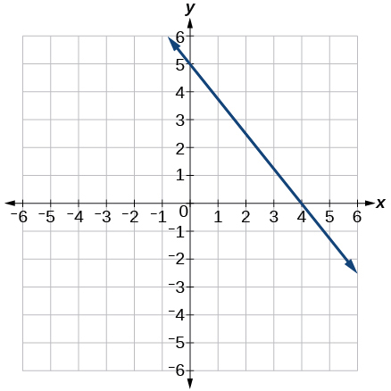
Solution (click to reveal)
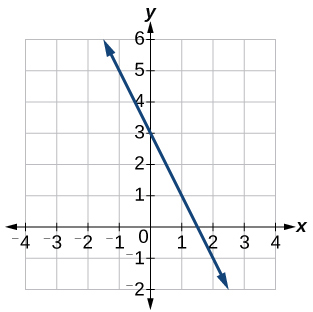
\(y = - \frac{5}{4}x + 5\)
60.
61.
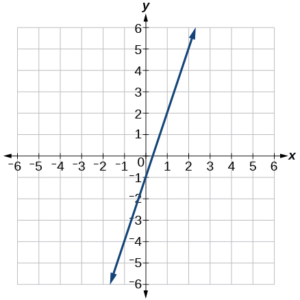
Solution (click to reveal)
\(y = 3x - 1\)
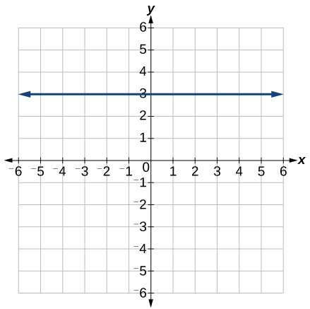
62.
63.
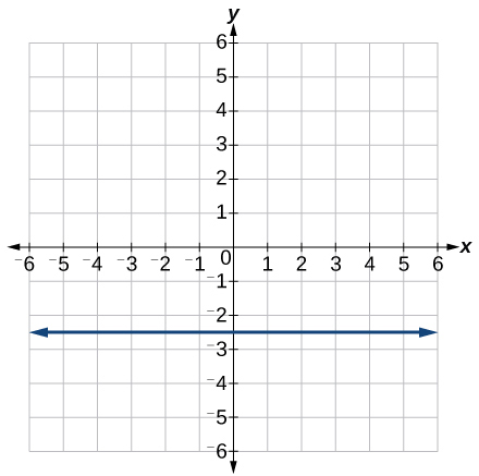
Solution (click to reveal)
\(y = - 2.5\)
For the following exercises, match the given linear equation with its graph in Figure 33.
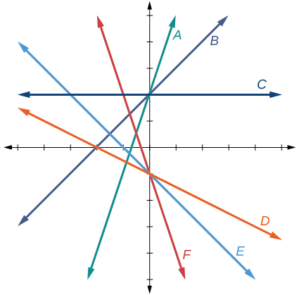
Figure 33
64. \(f(x) = - x - 1\)
65. \(f(x) = -3x - 1\)
Solution (click to reveal)
F
66. \(f(x) = - \frac{1}{2}x - 1\)
67. \(f(x) = 2\)
Solution (click to reveal)
C
68. \(f(x) = 2 + x\)
69. \(f(x) = 3x + 2\)
Solution (click to reveal)
A
For the following exercises, sketch a line with the given features.
70. An \(x\)-intercept of \((–4,\text{0})\) and \(y\)-intercept of \((0,\text{–2})\)
71. An \(x\)-intercept \((–2,\text{0})\) and \(y\)-intercept of \((0,\text{4})\)
Solution (click to reveal)
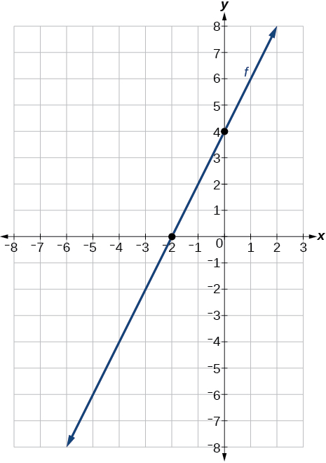
72. A \(y\)-intercept of \((0,\text{7})\) and slope \(- \frac{3}{2}\)
73. A \(y\)-intercept of \((0,\text{3})\) and slope \(\frac{2}{5}\)
Solution (click to reveal)
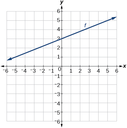
74. Passing through the points \((–6,\text{–2})\) and \((6,\text{–6})\)
75. Passing through the points \((–3,\text{–4})\) and \((3,\text{0})\)
Solution (click to reveal)
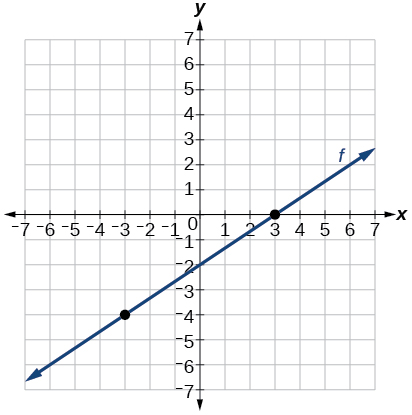
For the following exercises, sketch the graph of each equation.
76. \(f(x) = -2x - 1\)
77. \(f(x) = -3x + 2\)
Solution (click to reveal)
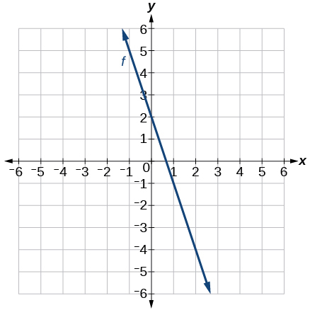
78. \(f(x) = \frac{1}{3}x + 2\)
79. \(f(x) = \frac{2}{3}x - 3\)
Solution (click to reveal)
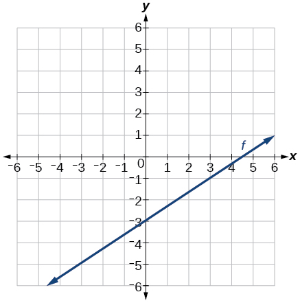
80. \(f(t) = 3 + 2t\)
81. \(p(t) = -2 + 3t\)
Solution (click to reveal)
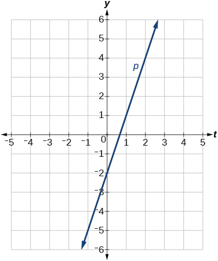
82. \(x = 3\)
83. \(x = -2\)
Solution (click to reveal)
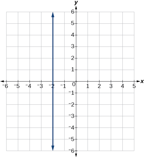
84. \(r(x) = 4\)
For the following exercises, write the equation of the line shown in the graph.
85.
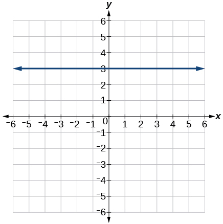
Solution (click to reveal)
\(y = \text{3}\)
86.
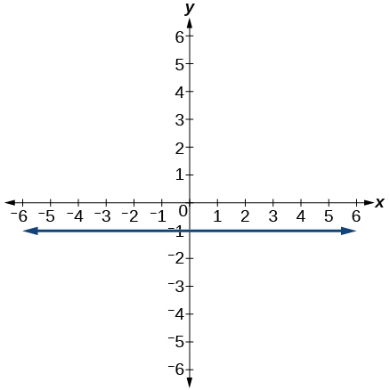
87.
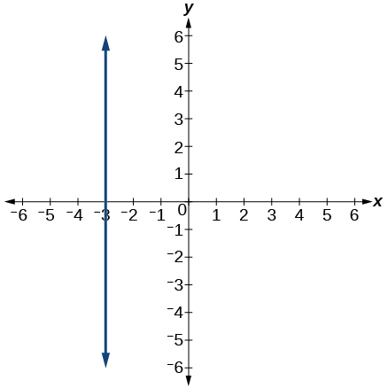
Solution (click to reveal)
\(x = - 3\)
88.
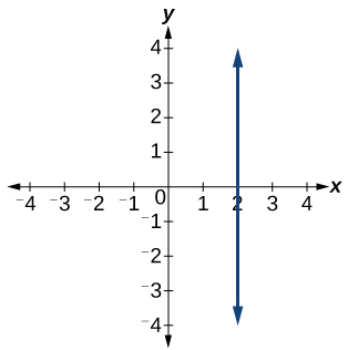
Numeric
For the following exercises, which of the tables could represent a linear function? For each that could be linear, find a linear equation that models the data.
89.
| \(x\) | 0 | 5 | 10 | 15 |
| \(g(x)\) | 5 | –10 | –25 | –40 |
Solution (click to reveal)
Linear, \(g(x) = - 3x + 5\)
90.
| \(x\) | 0 | 5 | 10 | 15 |
| \(h(x)\) | 5 | 30 | 105 | 230 |
91.
| \(x\) | 0 | 5 | 10 | 15 |
| \(f(x)\) | –5 | 20 | 45 | 70 |
Solution (click to reveal)
Linear, \(f(x) = 5x - 5\)
92.
| \(x\) | 5 | 10 | 20 | 25 |
| \(k(x)\) | 13 | 28 | 58 | 73 |
93.
| \(x\) | 0 | 2 | 4 | 6 |
| \(g(x)\) | 6 | –19 | –44 | –69 |
Solution (click to reveal)
Linear, \(g(x) = - \frac{25}{2}x + 6\)
94.
| \(x\) | 2 | 4 | 8 | 10 |
| \(h(x)\) | 13 | 23 | 43 | 53 |
95.
| \(x\) | 2 | 4 | 6 | 8 |
| \(f(x)\) | –4 | 16 | 36 | 56 |
Solution (click to reveal)
Linear, \(f(x) = 10x - 24\)
96.
| \(x\) | 0 | 2 | 6 | 8 |
| \(k(x)\) | 6 | 31 | 106 | 231 |
Technology
For the following exercises, use a calculator or graphing technology to complete the task.
97. If \(f\) is a linear function, \(f(0.1) = 11.5\) , and \(f(0.4) = –5.9\) , find an equation for the function.
Solution (click to reveal)
\(f(x) = - 58x + 17.3\)
98. Graph the function \(f\) on a domain of \(\lbrack –10,10\rbrack:f(x) = 0.02x - 0.01.\) Enter the function in a graphing utility. For the viewing window, set the minimum value of \(x\) to be \(-10\) and the maximum value of \(x\) to be \(10\) .
99. Graph the function \(f\) on a domain of \(\lbrack –10,10\rbrack:fx) = 2{,}500x + 4{,}000\)
Solution (click to reveal)
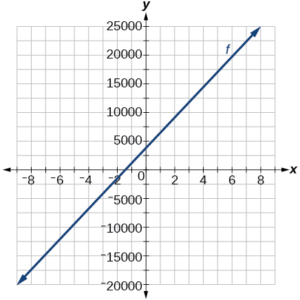
100. Table 3 shows the input, \(w,\) and output, \(k,\) for a linear function \(k.\)
ⓐ Fill in the missing values of the table. ⓑ Write the linear function
\(k,\) round to 3 decimal places.
| \(w\) | –10 | 5.5 | 67.5 | \(b\) |
| \(k\) | 30 | –26 | \(a\) | –44 |
Table 3
101. Table 4 shows the input, \(p,\) and output, \(q,\) for a linear function \(q.\)
ⓐ Fill in the missing values of the table. ⓑ Write the linear function
\(k.\)
| \(p\) | 0.5 | 0.8 | 12 | \(b\) |
| \(q\) | 400 | 700 | \(a\) | 1,000,000 |
Table 4
Solution (click to reveal)
ⓐ \(a = 11{,}900\text{,}\operatorname{}b = 1000.1\) ⓑ \(q(p) = 1000p–100\)
102. Graph the linear function \(f\) on a domain of \(\left\lbrack {- 10,10} \right\rbrack\) for the function whose slope is \(\frac{1}{8}\) and \(y\)-intercept is \(\frac{31}{16}.\) Label the points for the input values of \(-10\) and \(10.\)
103. Graph the linear function \(f\) on a domain of \(\left\lbrack {- 0.1,0.1} \right\rbrack\) for the function whose slope is 75 and \(y\)-intercept is \(-22.5.\) Label the points for the input values of \(-0.1\) and \(0.1.\)
Solution (click to reveal)
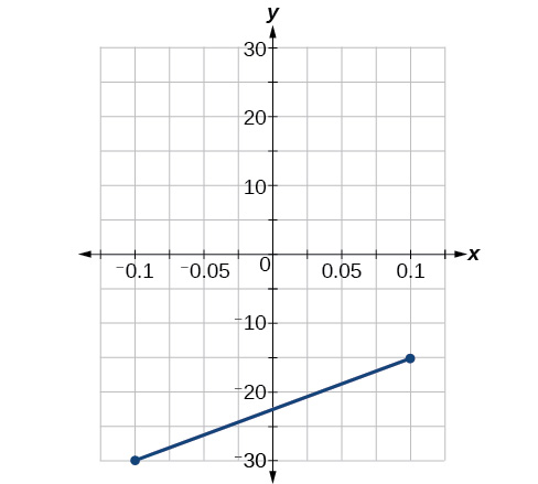
104. Graph the linear function \(f\) where \(f(x) = ax + b\) on the same set of axes on a domain of \(\left\lbrack {- 4,4} \right\rbrack\) for the following values of \(a\) and \(b.\)
ⓐ \(a = 2;b = 3\) ⓑ \(a = 2;b = 4\) ⓒ \(a = 2;b = –4\) ⓓ \(a = 2;b = –5\)
Extensions
105. Find the value of \(x\) if a linear function goes through the following points and has the following slope: \((x,2),(-4,6),\mspace{9mu} m = 3\)
Solution (click to reveal)
\(y = - \frac{16}{3}\)
106. Find the value ofy if a linear function goes through the following points and has the following slope: \((10,y),(25{,}100),\mspace{9mu} m = -5\)
107. Find the equation of the line that passes through the following points:
\(\left( {a,\mspace{9mu} b} \right)\) and \(\left( {a,\mspace{9mu} b + 1} \right)\)
Solution (click to reveal)
\(x = a\)
108. Find the equation of the line that passes through the following points:
\((2a,b)\) and \((a,b + 1)\)
109. Find the equation of the line that passes through the following points:
\((a,0)\) and \((c,d)\)
Solution (click to reveal)
\(y = \frac{d}{c–a}x–\frac{ad}{c–a}\)
110. Find the equation of the line parallel to the line \(g(x) = -0.\text{01}x\text{+2}\text{.01}\) through the point \((1,\text{2}).\)
111. Find the equation of the line perpendicular to the line \(g(x) = -0.\text{01}x\text{+2}\text{.01}\) through the point \((1,\text{2}).\)
Solution (click to reveal)
\(y = 100x–98\)
For the following exercises, use the functions \(f(x) = -0.\text{1}x\text{+200~and~}g(x) = 20x + 0.1.\)
112. Find the point of intersection of the lines \(f\) and \(g.\)
113. Where is \(f(x)\) greater than \(g(x)?\) Where is \(g(x)\) greater than \(f(x)?\)
Solution (click to reveal)
\(x < \frac{1999}{201}\text{,}x > \frac{1999}{201}\)
Real-World Applications
114. At noon, a barista notices that they have $20 in their tip jar. If the barista makes an average of $0.50 from each customer, how much will they have in the tip jar if they serve \(n\) more customers during the shift?
115. A gym membership with two personal training sessions costs $125, while gym membership with five personal training sessions costs $260. What is cost per session?
Solution (click to reveal)
$45 per training session.
116. A clothing business finds there is a linear relationship between the number of shirts, \(n,\) it can sell and the price, \(p,\) it can charge per shirt. In particular, historical data shows that 1,000 shirts can be sold at a price of \(\$ 30,\) while 3,000 shirts can be sold at a price of $22. Find a linear equation in the form \(p(n) = mn + b\) that gives the price \(p\) they can charge for \(n\) shirts.
117. A phone company charges for service according to the formula: \(C(n) = 24 + 0.1n,\) where \(n\) is the number of minutes talked, and \(C(n)\) is the monthly charge, in dollars. Find and interpret the rate of change and initial value.
Solution (click to reveal)
The rate of change is 0.1. For every additional minute talked, the monthly charge increases by $0.1 or 10 cents. The initial value is 24. When there are no minutes talked, initially the charge is $24.
118. A farmer finds there is a linear relationship between the number of bean stalks, \(n,\) she plants and the yield, \(y,\) each plant produces. When she plants 30 stalks, each plant yields 30 oz of beans. When she plants 34 stalks, each plant produces 28 oz of beans. Find a linear relationships in the form \(y = mn + b\) that gives the yield when \(n\) stalks are planted.
119. A city’s population in the year 1960 was 287,500. In 1989 the population was 275,900. Compute the rate of growth of the population and make a statement about the population rate of change in people per year.
Solution (click to reveal)
The slope is –400. this means for every year between 1960 and 1989, the population dropped by 400 per year in the city.
120. A town’s population has been growing linearly. In 2003, the population was 45,000, and the population has been growing by 1,700 people each year. Write an equation, \(P(t),\) for the population \(t\) years after 2003.
121. Suppose that average annual income (in dollars) for the years 1990 through 1999 is given by the linear function: \(I(x) = 1054x + 23{,}286\), where \(x\) is the number of years after 1990. Which of the following interprets the slope in the context of the problem?
ⓐ As of 1990, average annual income was $23,286.
ⓑ In the ten-year period from 1990–1999, average annual income increased by a total of $1,054.
ⓒ Each year in the decade of the 1990s, average annual income increased by $1,054.
ⓓ Average annual income rose to a level of $23,286 by the end of 1999.
Solution (click to reveal)
C
122. When temperature is 0 degrees Celsius, the Fahrenheit temperature is 32. When the Celsius temperature is 100, the corresponding Fahrenheit temperature is 212. Express the Fahrenheit temperature as a linear function of \(C,\) the Celsius temperature, \(F(C).\)
ⓐ Find the rate of change of Fahrenheit temperature for each unit change temperature of Celsius.
ⓑ Find and interpret \(F(28).\)
ⓒ Find and interpret \(F(–40).\)