11.5 Matrices and Matrix Operations

Figure 1 (credit: “SD Dirk,” Flickr)
Two club soccer teams, the Wildcats and the Mud Cats, are hoping to obtain new equipment for an upcoming season. Table 1 shows the needs of both teams.
| Wildcats | Mud Cats | |
|---|---|---|
| Goals | 6 | 10 |
| Balls | 30 | 24 |
| Jerseys | 14 | 20 |
Table 1
A goal costs $300; a ball costs $10; and a jersey costs $30. How can we find the total cost for the equipment needed for each team? In this section, we discover a method in which the data in the soccer equipment table can be displayed and used for calculating other information. Then, we will be able to calculate the cost of the equipment.
11.5.1 Finding the Sum and Difference of Two Matrices
To solve a problem like the one described for the soccer teams, we can use a matrix, which is a rectangular array of numbers. A row in a matrix is a set of numbers that are aligned horizontally. A column in a matrix is a set of numbers that are aligned vertically. Each number is an entry, sometimes called an element, of the matrix. Matrices (plural) are enclosed in [ ] or ( ), and are usually named with capital letters. For example, three matrices named \(A,B,\) and \(C\) are shown below.
\[A = \begin{bmatrix} 1 & 2 \\ 3 & 4 \end{bmatrix},B = \begin{bmatrix} 1 & 2 & 7 \\ 0 & -5 & 6 \\ 7 & 8 & 2 \end{bmatrix},C = \left\lbrack {\begin{matrix} -1 \\ {\mspace{9mu}\mspace{9mu}\mspace{9mu} 0} \\ {\mspace{9mu}\mspace{9mu}\mspace{9mu} 3} \end{matrix}\mspace{9mu}\mspace{9mu}\mspace{9mu}\mspace{9mu}\begin{matrix} 3 \\ 2 \\ 1 \end{matrix}} \right\rbrack\]
Describing Matrices
A matrix is often referred to by its size or dimensions: \(m \times n\) indicating \(m\) rows and \(n\) columns. Matrix entries are defined first by row and then by column. For example, to locate the entry in matrix \(A\) identified as \(a_{ij},\) we look for the entry in row \(i,\) column \(j.\) In matrix \(A\text{, }\) shown below, the entry in row 2, column 3 is \(a_{23}.\)
\[A = \begin{bmatrix} a_{11} & a_{12} & a_{13} \\ a_{21} & a_{22} & a_{23} \\ a_{31} & a_{32} & a_{33} \end{bmatrix}\]
A square matrix is a matrix with dimensions \(n \times n,\) meaning that it has the same number of rows as columns. The \(3 \times 3\) matrix above is an example of a square matrix.
A row matrix is a matrix consisting of one row with dimensions \(1 \times n.\)
\[\begin{bmatrix} a_{11} & a_{12} & a_{13} \end{bmatrix}\]
A column matrix is a matrix consisting of one column with dimensions \(m \times 1.\)
\[\begin{bmatrix} a_{11} \\ a_{21} \\ a_{31} \end{bmatrix}\]
A matrix may be used to represent a system of equations. In these cases, the numbers represent the coefficients of the variables in the system. Matrices often make solving systems of equations easier because they are not encumbered with variables. We will investigate this idea further in the next section, but first we will look at basic matrix operations.
Adding and Subtracting Matrices
We use matrices to list data or to represent systems. Because the entries are numbers, we can perform operations on matrices. We add or subtract matrices by adding or subtracting corresponding entries.
In order to do this, the entries must correspond. Therefore, addition and subtraction of matrices is only possible when the matrices have the same dimensions. We can add or subtract a \(3 \times 3\) matrix and another \(3 \times 3\) matrix, but we cannot add or subtract a \(2 \times 3\) matrix and a \(3 \times 3\) matrix because some entries in one matrix will not have a corresponding entry in the other matrix.
11.5.2 Finding Scalar Multiples of a Matrix
Besides adding and subtracting whole matrices, there are many situations in which we need to multiply a matrix by a constant called a scalar. Recall that a scalar is a real number quantity that has magnitude, but not direction. For example, time, temperature, and distance are scalar quantities. The process of scalar multiplication involves multiplying each entry in a matrix by a scalar. A scalar multiple is any entry of a matrix that results from scalar multiplication.
Consider a real-world scenario in which a university needs to add to its inventory of computers, computer tables, and chairs in two of the campus labs due to increased enrollment. They estimate that 15% more equipment is needed in both labs. The school’s current inventory is displayed in Table 2.
| Lab A | Lab B | |
|---|---|---|
| Computers | 15 | 27 |
| Computer Tables | 16 | 34 |
| Chairs | 16 | 34 |
Table 2
Converting the data to a matrix, we have
\[C_{2013} = \left\lbrack {\begin{matrix} 15 \\ 16 \\ 16 \end{matrix}\mspace{9mu}\mspace{9mu}\mspace{9mu}\mspace{9mu}\mspace{9mu}\mspace{9mu}\mspace{9mu}\begin{matrix} 27 \\ 34 \\ 34 \end{matrix}} \right\rbrack\]
To calculate how much computer equipment will be needed, we multiply all entries in matrix \(C\) by 0.15.
\[(0.15)C_{2013} = \left\lbrack {\begin{matrix} {(0.15)15} \\ {(0.15)16} \\ {(0.15)16} \end{matrix}\mspace{9mu}\mspace{9mu}\mspace{9mu}\mspace{9mu}\mspace{9mu}\mspace{9mu}\mspace{9mu}\mspace{9mu}\begin{matrix} {(0.15)27} \\ {(0.15)34} \\ {(0.15)34} \end{matrix}} \right\rbrack = \left\lbrack {\begin{matrix} 2.25 \\ 2.4 \\ 2.4 \end{matrix}\mspace{9mu}\mspace{9mu}\mspace{9mu}\mspace{9mu}\mspace{9mu}\begin{matrix} 4.05 \\ 5.1 \\ 5.1 \end{matrix}} \right\rbrack\]
We must round up to the next integer, so the amount of new equipment needed is
\[\left\lbrack {\begin{matrix} 3 \\ 3 \\ 3 \end{matrix}\mspace{9mu}\mspace{9mu}\mspace{9mu}\mspace{9mu}\mspace{9mu}\begin{matrix} 5 \\ 6 \\ 6 \end{matrix}} \right\rbrack\]
Adding the two matrices as shown below, we see the new inventory amounts.
\[\left\lbrack {\begin{matrix} 15 \\ 16 \\ 16 \end{matrix}\mspace{9mu}\mspace{9mu}\mspace{9mu}\mspace{9mu}\mspace{9mu}\mspace{9mu}\mspace{9mu}\begin{matrix} 27 \\ 34 \\ 34 \end{matrix}} \right\rbrack + \left\lbrack {\begin{matrix} 3 \\ 3 \\ 3 \end{matrix}\mspace{9mu}\mspace{9mu}\mspace{9mu}\mspace{9mu}\mspace{9mu}\begin{matrix} 5 \\ 6 \\ 6 \end{matrix}} \right\rbrack = \left\lbrack {\begin{matrix} 18 \\ 19 \\ 19 \end{matrix}\mspace{9mu}\mspace{9mu}\mspace{9mu}\mspace{9mu}\mspace{9mu}\begin{matrix} 32 \\ 40 \\ 40 \end{matrix}} \right\rbrack\]
This means
\[C_{2014} = \left\lbrack {\begin{matrix} 18 \\ 19 \\ 19 \end{matrix}\mspace{9mu}\mspace{9mu}\mspace{9mu}\mspace{9mu}\mspace{9mu}\begin{matrix} 32 \\ 40 \\ 40 \end{matrix}} \right\rbrack\]
Thus, Lab A will have 18 computers, 19 computer tables, and 19 chairs; Lab B will have 32 computers, 40 computer tables, and 40 chairs.
11.5.3 Finding the Product of Two Matrices
In addition to multiplying a matrix by a scalar, we can multiply two matrices. Finding the product of two matrices is only possible when the inner dimensions are the same, meaning that the number of columns of the first matrix is equal to the number of rows of the second matrix. If \(A\) is an \(m \times r\) matrix and \(B\) is an \(r \times n\) matrix, then the product matrix \(AB\) is an \(m \times n\) matrix. For example, the product \(AB\) is possible because the number of columns in \(A\) is the same as the number of rows in \(B.\) If the inner dimensions do not match, the product is not defined.
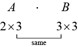
We multiply entries of \(A\) with entries of \(B\) according to a specific pattern as outlined below. The process of matrix multiplication becomes clearer when working a problem with real numbers.
To obtain the entries in row \(i\) of \(AB,\) we multiply the entries in row \(i\) of \(A\) by column \(j\) in \(B\) and add. For example, given matrices \(A\) and \(B,\) where the dimensions of \(A\) are \(2 \times 3\) and the dimensions of \(B\) are \(3 \times 3,\) the product of \(AB\) will be a \(2 \times 3\) matrix.
\[A = \left\lbrack \begin{array}{rrr} a_{11} & a_{12} & a_{13} \\ a_{21} & a_{22} & a_{23} \end{array} \right\rbrack\mspace{9mu}\text{and~}B = \left\lbrack \begin{array}{rrr} b_{11} & b_{12} & b_{13} \\ b_{21} & b_{22} & b_{23} \\ b_{31} & b_{32} & b_{33} \end{array} \right\rbrack\]
Multiply and add as follows to obtain the first entry of the product matrix \(AB.\)
- To obtain the entry in row 1, column 1 of \(AB,\) multiply the first row in \(A\) by the first column in \(B,\) and add.
\[\begin{bmatrix} a_{11} & a_{12} & a_{13} \end{bmatrix}\begin{bmatrix} b_{11} \\ b_{21} \\ b_{31} \end{bmatrix} = a_{11} \cdot b_{11} + a_{12} \cdot b_{21} + a_{13} \cdot b_{31}\]
- To obtain the entry in row 1, column 2 of \(AB,\) multiply the first row of \(A\) by the second column in \(B,\) and add.
\[\begin{bmatrix} a_{11} & a_{12} & a_{13} \end{bmatrix}\begin{bmatrix} b_{12} \\ b_{22} \\ b_{32} \end{bmatrix} = a_{11} \cdot b_{12} + a_{12} \cdot b_{22} + a_{13} \cdot b_{32}\]
- To obtain the entry in row 1, column 3 of \(AB,\) multiply the first row of \(A\) by the third column in \(B,\) and add.
\[\begin{bmatrix} a_{11} & a_{12} & a_{13} \end{bmatrix}\begin{bmatrix} b_{13} \\ b_{23} \\ b_{33} \end{bmatrix} = a_{11} \cdot b_{13} + a_{12} \cdot b_{23} + a_{13} \cdot b_{33}\]
We proceed the same way to obtain the second row of \(AB.\) In other words, row 2 of \(A\) times column 1 of \(B;\) row 2 of \(A\) times column 2 of \(B;\) row 2 of \(A\) times column 3 of \(B.\) When complete, the product matrix will be
\[AB = \left\lbrack {\begin{matrix} \begin{array}{l} {a_{11} \cdot b_{11} + a_{12} \cdot b_{21} + a_{13} \cdot b_{31}} \\ \end{array} \\ {a_{21} \cdot b_{11} + a_{22} \cdot b_{21} + a_{23} \cdot b_{31}} \end{matrix}\mspace{9mu}\mspace{9mu}\mspace{9mu}\mspace{9mu}\mspace{9mu}\mspace{9mu}\mspace{9mu}\mspace{9mu}\mspace{9mu}\begin{matrix} \begin{array}{l} {a_{11} \cdot b_{12} + a_{12} \cdot b_{22} + a_{13} \cdot b_{32}} \\ \end{array} \\ {a_{21} \cdot b_{12} + a_{22} \cdot b_{22} + a_{23} \cdot b_{32}} \end{matrix}\mspace{9mu}\mspace{9mu}\mspace{9mu}\mspace{9mu}\mspace{9mu}\mspace{9mu}\mspace{9mu}\mspace{9mu}\begin{matrix} \begin{array}{l} {a_{11} \cdot b_{13} + a_{12} \cdot b_{23} + a_{13} \cdot b_{33}} \\ \end{array} \\ {a_{21} \cdot b_{13} + a_{22} \cdot b_{23} + a_{23} \cdot b_{33}} \end{matrix}} \right\rbrack\]
Multiply matrix \(A\) and matrix \(B.\)
\[A = \begin{bmatrix} 1 & 2 \\ 3 & 4 \end{bmatrix}\mspace{9mu}\text{~and~~}B = \begin{bmatrix} 5 & 6 \\ 7 & 8 \end{bmatrix}\]
Solution (click to reveal)
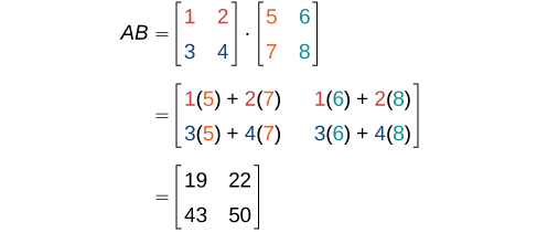
First, we check the dimensions of the matrices. Matrix \(A\) has dimensions \(2 \times 2\) and matrix \(B\) has dimensions \(2 \times 2.\) The inner dimensions are the same so we can perform the multiplication. The product will have the dimensions \(2 \times 2.\)
We perform the operations outlined previously.
Section Exercises
Verbal
1. Can we add any two matrices together? If so, explain why; if not, explain why not and give an example of two matrices that cannot be added together.
Solution (click to reveal)
No, they must have the same dimensions. An example would include two matrices of different dimensions. One cannot add the following two matrices because the first is a \(2 \times 2\) matrix and the second is a \(2 \times 3\) matrix. \(\begin{bmatrix} 1 & 2 \\ 3 & 4 \end{bmatrix} + \begin{bmatrix} 6 & 5 & 4 \\ 3 & 2 & 1 \end{bmatrix}\) has no sum.
2. Can we multiply any column matrix by any row matrix? Explain why or why not.
3. Can both the products \(AB\) and \(BA\) be defined? If so, explain how; if not, explain why.
Solution (click to reveal)
Yes, if the dimensions of \(A\) are \(m \times n\) and the dimensions of \(B\) are \(n \times m,\) both products will be defined.
4. Can any two matrices of the same size be multiplied? If so, explain why, and if not, explain why not and give an example of two matrices of the same size that cannot be multiplied together.
5. Does matrix multiplication commute? That is, does \(AB = BA?\) If so, prove why it does. If not, explain why it does not.
Solution (click to reveal)
Not necessarily. To find \(AB,\) we multiply the first row of \(A\) by the first column of \(B\) to get the first entry of \(AB.\) To find \(BA,\) we multiply the first row of \(B\) by the first column of \(A\) to get the first entry of \(BA.\) Thus, if those are unequal, then the matrix multiplication does not commute.
Algebraic
For the following exercises, use the matrices below and perform the matrix addition or subtraction. Indicate if the operation is undefined.
\[A = \begin{bmatrix} 1 & 3 \\ 0 & 7 \end{bmatrix},B = \begin{bmatrix} 2 & 14 \\ 22 & 6 \end{bmatrix},C = \begin{bmatrix} 1 & 5 \\ 8 & 92 \\ 12 & 6 \end{bmatrix},D = \begin{bmatrix} 10 & 14 \\ 7 & 2 \\ 5 & 61 \end{bmatrix},E = \begin{bmatrix} 6 & 12 \\ 14 & 5 \end{bmatrix},F = \begin{bmatrix} 0 & 9 \\ 78 & 17 \\ 15 & 4 \end{bmatrix}\]
6. \(A + B\)
7. \(C + D\)
Solution (click to reveal)
\(\begin{bmatrix} 11 & 19 \\ 15 & 94 \\ 17 & 67 \end{bmatrix}\)
8. \(A + C\)
9. \(B - E\)
Solution (click to reveal)
\(\begin{bmatrix} -4 & 2 \\ 8 & 1 \end{bmatrix}\)
10. \(C + F\)
11. \(D - B\)
Solution (click to reveal)
Undidentified; dimensions do not match
For the following exercises, use the matrices below to perform scalar multiplication.
\[A = \left\lbrack \begin{array}{rr} 4 & 6 \\ 13 & 12 \end{array} \right\rbrack,B = \left\lbrack \begin{array}{rr} 3 & 9 \\ 21 & 12 \\ 0 & 64 \end{array} \right\rbrack,C = \left\lbrack \begin{array}{rrrr} 16 & 3 & 7 & 18 \\ 90 & 5 & 3 & 29 \end{array} \right\rbrack,D = \left\lbrack \begin{array}{rrr} 18 & 12 & 13 \\ 8 & 14 & 6 \\ 7 & 4 & 21 \end{array} \right\rbrack\]
12. \(5A\)
13. \(3B\)
Solution (click to reveal)
\(\begin{bmatrix} 9 & 27 \\ 63 & 36 \\ 0 & 192 \end{bmatrix}\)
14. \(-2B\)
15. \(-4C\)
Solution (click to reveal)
\(\begin{bmatrix} -64 & -12 & -28 & -72 \\ -360 & -20 & -12 & -116 \end{bmatrix}\)
16. \(\frac{1}{2}C\)
17. \(100D\)
Solution (click to reveal)
\(\begin{bmatrix} {1{,}800} & {1{,}200} & {1{,}300} \\ 800 & {1{,}400} & 600 \\ 700 & 400 & {2{,}100} \end{bmatrix}\)
For the following exercises, use the matrices below to perform matrix multiplication.
\[A = \left\lbrack \begin{array}{rr} -1 & 5 \\ 3 & 2 \end{array} \right\rbrack,B = \left\lbrack \begin{array}{rrr} 3 & 6 & 4 \\ -8 & 0 & 12 \end{array} \right\rbrack,C = \left\lbrack \begin{array}{rr} 4 & 10 \\ -2 & 6 \\ 5 & 9 \end{array} \right\rbrack,D = \left\lbrack \begin{array}{rrr} 2 & -3 & 12 \\ 9 & 3 & 1 \\ 0 & 8 & -10 \end{array} \right\rbrack\]
18. \(AB\)
19. \(BC\)
Solution (click to reveal)
\(\begin{bmatrix} 20 & 102 \\ 28 & 28 \end{bmatrix}\)
20. \(CA\)
21. \(BD\)
Solution (click to reveal)
\(\begin{bmatrix} 60 & 41 & 2 \\ -16 & 120 & -216 \end{bmatrix}\)
22. \(DC\)
23. \(CB\)
Solution (click to reveal)
\(\begin{bmatrix} -68 & 24 & 136 \\ -54 & -12 & 64 \\ -57 & 30 & 128 \end{bmatrix}\)
For the following exercises, use the matrices below to perform the indicated operation if possible. If not possible, explain why the operation cannot be performed.
\[A = \left\lbrack \begin{array}{rr} 2 & -5 \\ 6 & 7 \end{array} \right\rbrack,B = \left\lbrack \begin{array}{rr} -9 & 6 \\ -4 & 2 \end{array} \right\rbrack,C = \left\lbrack \begin{array}{rr} 0 & 9 \\ 7 & 1 \end{array} \right\rbrack,D = \left\lbrack \begin{array}{rrr} -8 & 7 & -5 \\ 4 & 3 & 2 \\ 0 & 9 & 2 \end{array} \right\rbrack,E = \left\lbrack \begin{array}{rrr} 4 & 5 & 3 \\ 7 & -6 & -5 \\ 1 & 0 & 9 \end{array} \right\rbrack\]
24. \(A + B - C\)
25. \(4A + 5D\)
Solution (click to reveal)
Undefined; dimensions do not match.
26. \(2C + B\)
27. \(3D + 4E\)
Solution (click to reveal)
\(\begin{bmatrix} -8 & 41 & -3 \\ 40 & -15 & -14 \\ 4 & 27 & 42 \end{bmatrix}\)
28. \(C-0.5D\)
29. \(100D-10E\)
Solution (click to reveal)
\(\begin{bmatrix} -840 & 650 & -530 \\ 330 & 360 & 250 \\ -10 & 900 & 110 \end{bmatrix}\)
For the following exercises, use the matrices below to perform the indicated operation if possible. If not possible, explain why the operation cannot be performed. (Hint: \(A^{2} = A \cdot A\) )
\[A = \left\lbrack \begin{array}{rr} -10 & 20 \\ 5 & 25 \end{array} \right\rbrack,B = \left\lbrack \begin{array}{rr} 40 & 10 \\ -20 & 30 \end{array} \right\rbrack,C = \left\lbrack \begin{array}{rr} -1 & 0 \\ 0 & -1 \\ 1 & 0 \end{array} \right\rbrack\]
30. \(AB\)
31. \(BA\)
Solution (click to reveal)
\(\begin{bmatrix} -350 & {1{,}050} \\ 350 & 350 \end{bmatrix}\)
32. \(CA\)
33. \(BC\)
Solution (click to reveal)
Undefined; inner dimensions do not match.
34. \(A^{2}\)
35. \(B^{2}\)
Solution (click to reveal)
\(\begin{bmatrix} {1{,}400} & 700 \\ {-1{,}400} & 700 \end{bmatrix}\)
36. \(C^{2}\)
37. \(B^{2}A^{2}\)
Solution (click to reveal)
\(\begin{bmatrix} {332{,}500} & {927{,}500} \\ {-227{,}500} & {87{,}500} \end{bmatrix}\)
38. \(A^{2}B^{2}\)
39. \({(AB)}^{2}\)
Solution (click to reveal)
\(\begin{bmatrix} {490{,}000} & 0 \\ 0 & {490{,}000} \end{bmatrix}\)
40. \({(BA)}^{2}\)
For the following exercises, use the matrices below to perform the indicated operation if possible. If not possible, explain why the operation cannot be performed. (Hint: \(A^{2} = A \cdot A\) )
\[A = \left\lbrack \begin{array}{rr} 1 & 0 \\ 2 & 3 \end{array} \right\rbrack,B = \left\lbrack \begin{array}{rrr} -2 & 3 & 4 \\ -1 & 1 & -5 \end{array} \right\rbrack,C = \left\lbrack \begin{array}{rr} 0.5 & 0.1 \\ 1 & 0.2 \\ -0.5 & 0.3 \end{array} \right\rbrack,D = \left\lbrack \begin{array}{rrr} 1 & 0 & -1 \\ -6 & 7 & 5 \\ 4 & 2 & 1 \end{array} \right\rbrack\]
41. \(AB\)
Solution (click to reveal)
\(\begin{bmatrix} -2 & 3 & 4 \\ -7 & 9 & -7 \end{bmatrix}\)
42. \(BA\)
43. \(BD\)
Solution (click to reveal)
\(\begin{bmatrix} -4 & 29 & 21 \\ -27 & -3 & 1 \end{bmatrix}\)
44. \(DC\)
45. \(D^{2}\)
Solution (click to reveal)
\(\begin{bmatrix} -3 & -2 & -2 \\ -28 & 59 & 46 \\ -4 & 16 & 7 \end{bmatrix}\)
46. \(A^{2}\)
47. \(D^{3}\)
Solution (click to reveal)
\(\begin{bmatrix} 1 & -18 & -9 \\ -198 & 505 & 369 \\ -72 & 126 & 91 \end{bmatrix}\)
48. \((AB)C\)
49. \(A(BC)\)
Solution (click to reveal)
\(\begin{bmatrix} 0 & 1.6 \\ 9 & -1 \end{bmatrix}\)
Technology
For the following exercises, use the matrices below to perform the indicated operation if possible. If not possible, explain why the operation cannot be performed. Use a calculator to verify your solution.
\[A = \left\lbrack \begin{array}{rrr} -2 & 0 & 9 \\ 1 & 8 & -3 \\ 0.5 & 4 & 5 \end{array} \right\rbrack,B = \left\lbrack \begin{array}{rrr} 0.5 & 3 & 0 \\ -4 & 1 & 6 \\ 8 & 7 & 2 \end{array} \right\rbrack,C = \left\lbrack \begin{array}{rrr} 1 & 0 & 1 \\ 0 & 1 & 0 \\ 1 & 0 & 1 \end{array} \right\rbrack\]
50. \(AB\)
51. \(BA\)
Solution (click to reveal)
\(\begin{bmatrix} 2 & 24 & -4.5 \\ 12 & 32 & -9 \\ -8 & 64 & 61 \end{bmatrix}\)
52. \(CA\)
53. \(BC\)
Solution (click to reveal)
\(\begin{bmatrix} 0.5 & 3 & 0.5 \\ 2 & 1 & 2 \\ 10 & 7 & 10 \end{bmatrix}\)
54. \(ABC\)
Extensions
For the following exercises, use the matrix below to perform the indicated operation on the given matrix.
\[B = \left\lbrack \begin{array}{rrr} 1 & 0 & 0 \\ 0 & 0 & 1 \\ 0 & 1 & 0 \end{array} \right\rbrack\]
55. \(B^{2}\)
Solution (click to reveal)
\(\begin{bmatrix} 1 & 0 & 0 \\ 0 & 1 & 0 \\ 0 & 0 & 1 \end{bmatrix}\)
56. \(B^{3}\)
57. \(B^{4}\)
Solution (click to reveal)
\(\begin{bmatrix} 1 & 0 & 0 \\ 0 & 1 & 0 \\ 0 & 0 & 1 \end{bmatrix}\)
58. \(B^{5}\)
59. Using the above questions, find a formula for \(B^{n}.\) Test the formula for \(B^{201}\) and \(B^{202},\) using a calculator.
Solution (click to reveal)
\(B^{n} = \left\{ \begin{array}{l} {\left\lbrack \begin{array}{lll} 1 & 0 & 0 \\ 0 & 1 & 0 \\ 0 & 0 & 1 \end{array} \right\rbrack,\quad n\mspace{9mu}\text{even,}} \\ {\left\lbrack \begin{array}{lll} 1 & 0 & 0 \\ 0 & 0 & 1 \\ 0 & 1 & 0 \end{array} \right\rbrack,\quad n\mspace{9mu}\text{odd}\text{.}} \end{array} \right.\)