10.7 Parametric Equations: Graphs
While not every fan (or team manager) appreciates it, baseball and many other sports have become dependent on analytics, which involve complex data recording and quantitative evaluation used to understand and predict behavior. The earliest influence of analytics was mostly statistical; more recently, physics and other sciences have come into play. Foremost among these is the focus on launch angle and exit velocity, which when at certain values can almost guarantee a home run. On the other hand, emphasis on launch angle and focusing on home runs rather than overall hitting results in far more outs. Consider the following situation: it is the bottom of the ninth inning, with two outs and two players on base. The home team is losing by two runs. The batter swings and hits the baseball at 140 feet per second and at an angle of approximately \(45{^\circ}\) to the horizontal. How far will the ball travel? Will it clear the fence for a game-winning home run? The outcome may depend partly on other factors (for example, the wind), but mathematicians can model the path of a projectile and predict approximately how far it will travel using parametric equations. In this section, we’ll discuss parametric equations and some common applications, such as projectile motion problems.
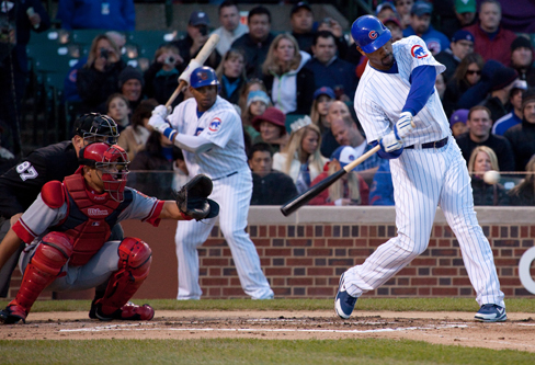
Figure 1 Parametric equations can model the path of a projectile. (credit: Paul Kreher, Flickr)
10.7.1 Graphing Parametric Equations by Plotting Points
In lieu of a graphing calculator or a computer graphing program, plotting points to represent the graph of an equation is the standard method. As long as we are careful in calculating the values, point-plotting is highly dependable.
Sketch the graph of the parametric equations \(x(t) = t^{2} + 1,\) \(y(t) = 2 + t.\)
Solution (click to reveal)
Construct a table of values for \(t,x(t),\) and \(y(t),\) as in Table 1, and plot the points in a plane.
| \(t\) | \(x(t) = t^{2} + 1\) | \(y(t) = 2 + t\) |
|---|---|---|
| \(- 5\) | \(26\) | \(- 3\) |
| \(- 4\) | \(17\) | \(- 2\) |
| \(- 3\) | \(10\) | \(- 1\) |
| \(- 2\) | \(5\) | \(0\) |
| \(- 1\) | \(2\) | \(1\) |
| \(0\) | \(1\) | \(2\) |
| \(1\) | \(2\) | \(3\) |
| \(2\) | \(5\) | \(4\) |
| \(3\) | \(10\) | \(5\) |
| \(4\) | \(17\) | \(6\) |
| \(5\) | \(26\) | \(7\) |
Table 1
The graph is a parabola with vertex at the point \(\left( {1,2} \right),\) opening to the right. See Figure 2.
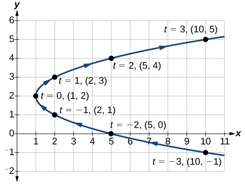
Figure 2
As values for \(t\) progress in a positive direction from 0 to 5, the plotted points trace out the top half of the parabola. As values of \(t\) become negative, they trace out the lower half of the parabola. There are no restrictions on the domain. The arrows indicate direction according to increasing values of \(t.\) The graph does not represent a function, as it will fail the vertical line test. The graph is drawn in two parts: the positive values for \(t,\) and the negative values for \(t.\)
Sketch the graph of the parametric equations \(x = \sqrt{t},\) \(y = 2t + 3,\) \(0 \leq t \leq 3.\)
Solution (click to reveal)
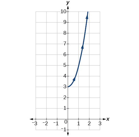
Construct a table of values for the given parametric equations and sketch the graph:
\[\begin{array}{l} {x = 2\cos\; t} \\ {y = 4\sin\; t} \end{array}\]
Solution (click to reveal)
Construct a table like that in Table 2 using angle measure in radians as inputs for \(t,\) and evaluating \(x\) and \(y.\) Using angles with known sine and cosine values for \(t\) makes calculations easier.
| \(t\) | \(x = 2\cos\; t\) | \(y = 4\sin\; t\) |
|---|---|---|
| 0 | \(x = 2\cos(0) = 2\) | \(y = 4\sin(0) = 0\) |
| \(\frac{\pi}{6}\) | \(x = 2\cos\left( \frac{\pi}{6} \right) = \sqrt{3}\) | \(y = 4\sin\left( \frac{\pi}{6} \right) = 2\) |
| \(\frac{\pi}{3}\) | \(x = 2\cos\left( \frac{\pi}{3} \right) = 1\) | \(y = 4\sin\left( \frac{\pi}{3} \right) = 2\sqrt{3}\) |
| \(\frac{\pi}{2}\) | \(x = 2\cos\left( \frac{\pi}{2} \right) = 0\) | \(y = 4\sin\left( \frac{\pi}{2} \right) = 4\) |
| \(\frac{2\pi}{3}\) | \(x = 2\cos\left( \frac{2\pi}{3} \right) = - 1\) | \(y = 4\sin\left( \frac{2\pi}{3} \right) = 2\sqrt{3}\) |
| \(\frac{5\pi}{6}\) | \(x = 2\cos\left( \frac{5\pi}{6} \right) = - \sqrt{3}\) | \(y = 4\sin\left( \frac{5\pi}{6} \right) = 2\) |
| \(\pi\) | \(x = 2\cos(\pi) = - 2\) | \(y = 4\sin(\pi) = 0\) |
| \(\frac{7\pi}{6}\) | \(x = 2\cos\left( \frac{7\pi}{6} \right) = - \sqrt{3}\) | \(y = 4\sin\left( \frac{7\pi}{6} \right) = - 2\) |
| \(\frac{4\pi}{3}\) | \(x = 2\cos\left( \frac{4\pi}{3} \right) = - 1\) | \(y = 4\sin\left( \frac{4\pi}{3} \right) = - 2\sqrt{3}\) |
| \(\frac{3\pi}{2}\) | \(x = 2\cos\left( \frac{3\pi}{2} \right) = 0\) | \(y = 4\sin\left( \frac{3\pi}{2} \right) = - 4\) |
| \(\frac{5\pi}{3}\) | \(x = 2\cos\left( \frac{5\pi}{3} \right) = 1\) | \(y = 4\sin\left( \frac{5\pi}{3} \right) = - 2\sqrt{3}\) |
| \(\frac{11\pi}{6}\) | \(x = 2\cos\left( \frac{11\pi}{6} \right) = \sqrt{3}\) | \(y = 4\sin\left( \frac{11\pi}{6} \right) = - 2\) |
| \(2\pi\) | \(x = 2\cos(2\pi) = 2\) | \(y = 4\sin\left( {2\pi} \right) = 0\) |
Table 2
Figure 3 shows the graph.
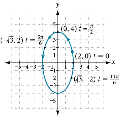
Figure 3
By the symmetry shown in the values of \(x\) and \(y,\) we see that the parametric equations represent an ellipse. The ellipse is mapped in a counterclockwise direction as shown by the arrows indicating increasing \(t\) values.
We have seen that parametric equations can be graphed by plotting points. However, a graphing calculator will save some time and reveal nuances in a graph that may be too tedious to discover using only hand calculations.
Make sure to change the mode on the calculator to parametric (PAR). To confirm, the \(Y =\) window should show
\[\begin{matrix} {X_{1T} =} \\ {Y_{1T} =} \end{matrix}\]
instead of \(Y_{1} = .\)
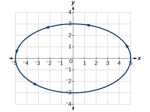
Graph the parametric equations: \(x = 5\cos\; t,\) \(y = 3\sin\; t.\)
Solution (click to reveal)
Graph the parametric equations \(x = 5\cos\; t\) and \(y = 2\sin\; t.\) First, construct the graph using data points generated from the parametric form. Then graph the rectangular form of the equation. Compare the two graphs.
Solution (click to reveal)
Construct a table of values like that in Table 3.
| \(t\) | \(x = 5\cos\; t\) | \(y = 2\sin\; t\) |
|---|---|---|
| \(\text{0}\) | \(x = 5\cos(0) = 5\) | \(y = 2\sin(0) = 0\) |
| \(\text{1}\) | \(x = 5\cos(1) \approx 2.7\) | \(y = 2\sin(1) \approx 1.7\) |
| \(\text{2}\) | \(x = 5\cos(2) \approx -2.1\) | \(y = 2\sin(2) \approx 1.8\) |
| \(\text{3}\) | \(x = 5\cos(3) \approx -4.95\) | \(y = 2\sin(3) \approx 0.28\) |
| \(\text{4}\) | \(x = 5\cos(4) \approx -3.3\) | \(y = 2\sin(4) \approx -1.5\) |
| \(\text{5}\) | \(x = 5\cos(5) \approx 1.4\) | \(y = 2\sin(5) \approx -1.9\) |
| \(-1\) | \(x = 5\cos(-1) \approx 2.7\) | \(y = 2\sin(-1) \approx -1.7\) |
| \(-2\) | \(x = 5\cos(-2) \approx -2.1\) | \(y = 2\sin(-2) \approx -1.8\) |
| \(-3\) | \(x = 5\cos(-3) \approx -4.95\) | \(y = 2\sin(-3) \approx -0.28\) |
| \(-4\) | \(x = 5\cos(-4) \approx -3.3\) | \(y = 2\sin(-4) \approx 1.5\) |
| \(-5\) | \(x = 5\cos(-5) \approx 1.4\) | \(y = 2\sin(-5) \approx 1.9\) |
Table 3
Plot the \(\left( {x,y} \right)\) values from the table. See Figure 4.
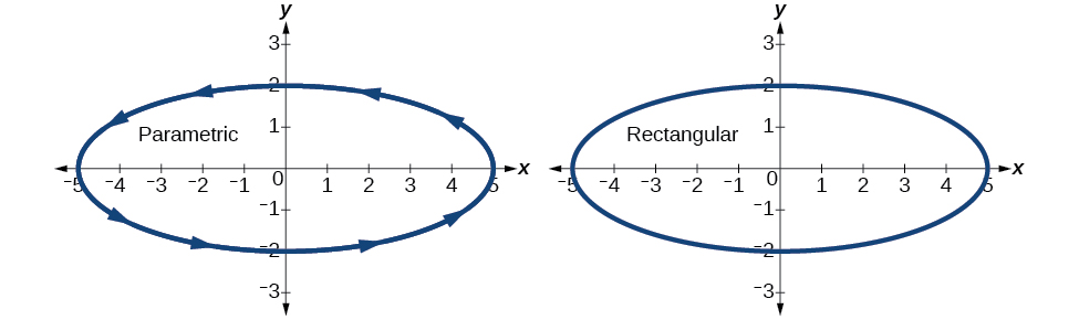
Figure 4
Next, translate the parametric equations to rectangular form. To do this, we solve for \(t\) in either \(x(t)\) or \(y(t),\) and then substitute the expression for \(t\) in the other equation. The result will be a function \(y(x)\) if solving for \(t\) as a function of \(x,\) or \(x(y)\) if solving for \(t\) as a function of \(y.\)
\[\begin{array}{ll} {x = 5\cos\; t} & \\ {\frac{x}{5} = \cos\; t} & {\text{Solve~for~}\cos\; t.} \\ {y = 2\sin\; t\begin{array}{llll} & & & \end{array}\mspace{9mu}} & {\text{Solve~for~}\sin\; t.} \\ {\frac{y}{2} = \sin\; t} & \end{array}\]
Then, use the Pythagorean Theorem.
\[\begin{array}{r} {\cos^{2}t + \sin^{2}t = 1} \\ {\left( \frac{x}{5} \right)^{2} + \left( \frac{y}{2} \right)^{2} = 1} \\ {\frac{x^{2}}{25} + \frac{y^{2}}{4} = 1} \end{array}\]
In Figure 5, the data from the parametric equations and the rectangular equation are plotted together. The parametric equations are plotted in blue; the graph for the rectangular equation is drawn on top of the parametric in a dashed style colored red. Clearly, both forms produce the same graph.
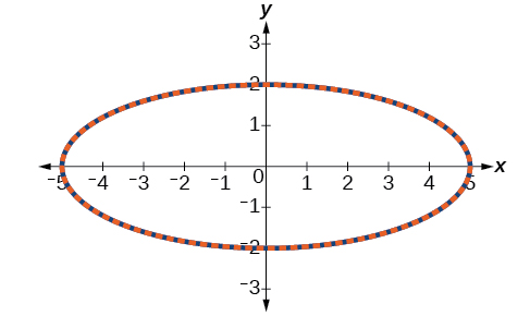
Figure 5
Graph the parametric equations \(x = t + 1\) and \(y = \sqrt{t},\) \(t \geq 0,\) and the rectangular equivalent \(y = \sqrt{x - 1}\) on the same coordinate system.
Solution (click to reveal)
Construct a table of values for the parametric equations, as we did in the previous example, and graph \(y = \sqrt{t},\) \(t \geq 0\) on the same grid, as in Figure 6.
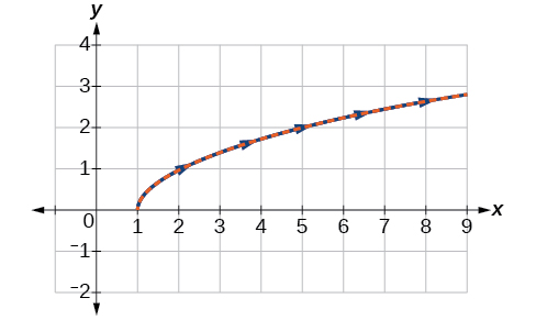
Figure 6
With the domain on \(t\) restricted, we only plot positive values of \(t.\) The parametric data is graphed in blue and the graph of the rectangular equation is dashed in red. Once again, we see that the two forms overlap.
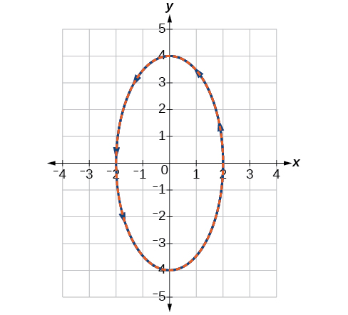
Sketch the graph of the parametric equations \(x = 2\cos\;\theta\mspace{9mu}\text{and}\mspace{9mu} y = 4\sin\;\theta,\) along with the rectangular equation on the same grid.
Solution (click to reveal)
The graph of the parametric equations is in red and the graph of the rectangular equation is drawn in blue dots on top of the parametric equations.
10.7.2 Applications of Parametric Equations
Many of the advantages of parametric equations become obvious when applied to solving real-world problems. Although rectangular equations in \(x\) and \(y\) give an overall picture of an object’s path, they do not reveal the position of an object at a specific time. Parametric equations, however, illustrate how the values of \(x\) and \(y\) change depending on \(t\), as the location of a moving object at a particular time.
A common application of parametric equations is solving problems involving projectile motion. In this type of motion, an object is propelled forward in an upward direction forming an angle of \(\theta\) to the horizontal, with an initial speed of \(v_{0},\) and at a height \(h\) above the horizontal.
The path of an object propelled at an inclination of \(\theta\) to the horizontal, with initial speed \(v_{0},\) and at a height \(h\) above the horizontal, is given by
\[\begin{array}{l} {x = (v_{0}\cos\theta)t\text{~~}} \\ {y = - \frac{1}{2}gt^{2} + (v_{0}\sin\theta)t + h} \end{array}\]
where \(g\) accounts for the effects of gravity and \(h\) is the initial height of the object. Depending on the units involved in the problem, use \(g = 32\;\text{ft}\text{/}\text{s}^{2}\) or \(g = 9.8\;\text{m}\text{/}\text{s}^{2}.\) The equation for \(x\) gives horizontal distance, and the equation for \(y\) gives the vertical distance.
Solve the problem presented at the beginning of this section. Does the batter hit the game-winning home run? Assume that the ball is hit with an initial velocity of 140 feet per second at an angle of \(45{^\circ}\) to the horizontal, making contact 3 feet above the ground.
ⓐ Find the parametric equations to model the path of the baseball.
ⓑ Where is the ball after 2 seconds?
ⓒ How long is the ball in the air?
ⓓ Is it a home run?
Solution (click to reveal)
ⓐ Use the formulas to set up the equations. The horizontal position is found using the parametric equation for \(\; x.\) Thus,
\[\begin{array}{l} {x = (v_{0}\cos\;\theta)t} \\ {x = (140\cos(45{^\circ}))t} \end{array}\]
The vertical position is found using the parametric equation for \(y.\) Thus,
\[\begin{array}{l} {y = - 16t^{2} + (v_{0}\sin\;\theta)t + h} \\ {y = - 16t^{2} + (140\sin(45{^\circ}))t + 3} \end{array}\]
ⓑ Substitute 2 into the equations to find the horizontal and vertical positions of the ball.
\[\begin{array}{l} {x = (140\cos(45{^\circ}))(2)} \\ {x = 198\text{~feet}} \\ \\ {y = - 16{(2)}^{2} + (140\sin(45{^\circ}))(2) + 3} \\ {y = 137\text{~feet}} \end{array}\]
After 2 seconds, the ball is 198 feet away from the batter’s box and 137 feet above the ground.
ⓒ To calculate how long the ball is in the air, we have to find out when it will hit ground, or when \(y = 0.\) Thus,
\[\begin{array}{ll} {y = - 16t^{2} + \left( {140\sin(45^{\circ})} \right)t + 3} & \\ {y = 0} & {\text{Set~}y(t) = 0\text{~and~solve~the~quadratic}.} \\ {t = 6.2173} & \end{array}\]
When \(t = 6.2173\) seconds, the ball has hit the ground. (The quadratic equation can be solved in various ways, but this problem was solved using a computer math program.)
ⓓ We cannot confirm that the hit was a home run without considering the size of the outfield, which varies from field to field. However, for simplicity’s sake, let’s assume that the outfield wall is 400 feet from home plate in the deepest part of the park. Let’s also assume that the wall is 10 feet high. In order to determine whether the ball clears the wall, we need to calculate how high the ball is when \(x\) = 400 feet. So we will set \(x\) = 400, solve for \(t,\) and input \(t\) into \(y.\)
\[\begin{matrix} \begin{array}{l} {x = \left( {140\cos(45{^\circ})} \right)t} \\ {400 = \left( {140\cos(45{^\circ})} \right)t} \\ {t = 4.04} \end{array} \\ \\ \begin{array}{l} {y = - 16{(4.04)}^{2} + \left( {140\sin(45{^\circ})} \right)(4.04) + 3} \\ {y = 141.8} \end{array} \end{matrix}\]
The ball is 141.8 feet in the air when it soars out of the ballpark. It was indeed a home run. See Figure 7.
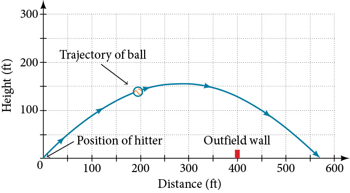
Figure 7
Section Exercises
Verbal
1. What are two methods used to graph parametric equations?
Solution (click to reveal)
plotting points with the orientation arrow and a graphing calculator
2. What is one difference in point-plotting parametric equations compared to Cartesian equations?
3. Why are some graphs drawn with arrows?
Solution (click to reveal)
The arrows show the orientation, the direction of motion according to increasing values of \(t.\)
4. Name a few common types of graphs of parametric equations.
5. Why are parametric graphs important in understanding projectile motion?
Solution (click to reveal)
The parametric equations show the different vertical and horizontal motions over time.
Graphical
For the following exercises, graph each set of parametric equations by making a table of values. Include the orientation on the graph.
6. \(\left\{ \begin{array}{l} {x(t) = t} \\ {y(t) = t^{2} - 1} \end{array} \right.\)
| \(t\) | \(- 3\) | \(- 2\) | \(- 1\) | \(0\) | \(1\) | \(2\) | \(3\) |
| \(x\) | |||||||
| \(y\) |
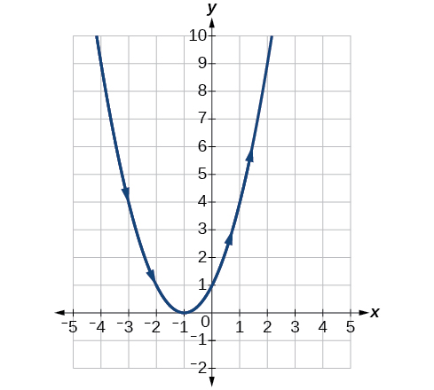
7. \(\left\{ \begin{array}{l} {x(t) = t - 1} \\ {y(t) = t^{2}} \end{array} \right.\)
| \(t\) | \(- 3\) | \(- 2\) | \(- 1\) | \(0\) | \(1\) | \(2\) |
| \(x\) | ||||||
| \(y\) |
Solution (click to reveal)
8. \(\left\{ \begin{array}{l} {x(t) = 2 + t} \\ {y(t) = 3 - 2t} \end{array} \right.\)
| \(t\) | \(- 2\) | \(- 1\) | \(0\) | \(1\) | \(2\) | \(3\) |
| \(x\) | ||||||
| \(y\) |
9. \(\left\{ \begin{array}{l} {x(t) = - 2 - 2t} \\ {y(t) = 3 + t} \end{array} \right.\)
| \(t\) | \(- 3\) | \(- 2\) | \(- 1\) | \(0\) | \(1\) |
| \(x\) | |||||
| \(y\) |
Solution (click to reveal)
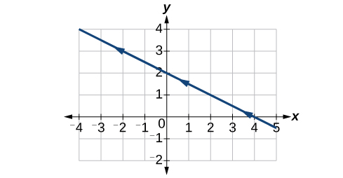
10. \(\left\{ \begin{array}{l} {x(t) = t^{3}} \\ {y(t) = t + 2} \end{array} \right.\)
| \(t\) | \(- 2\) | \(- 1\) | \(0\) | \(1\) | \(2\) |
| \(x\) | |||||
| \(y\) |
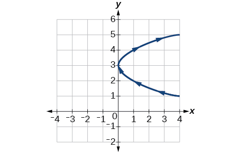
11. \(\left\{ \begin{array}{l} {x(t) = t^{2}} \\ {y(t) = t + 3} \end{array} \right.\)
| \(t\) | \(- 2\) | \(- 1\) | \(0\) | \(1\) | \(2\) |
| \(x\) | |||||
| \(y\) |
Solution (click to reveal)
For the following exercises, sketch the curve and include the orientation.
12. \(\left\{ \begin{array}{l} {x(t) = t} \\ {y(t) = \sqrt{t}} \end{array} \right.\)
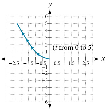
13. \(\left\{ \begin{array}{l} {x(t) = - \;\sqrt{t}} \\ {y(t) = t} \end{array} \right.\)
Solution (click to reveal)
14. \(\left\{ \begin{array}{l} {x(t) = 5 - |t|} \\ {y(t) = t + 2} \end{array} \right.\)
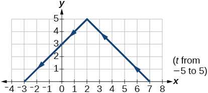
15. \(\left\{ \begin{array}{l} {x(t) = - t + 2} \\ {y(t) = 5 - |t|} \end{array} \right.\)
Solution (click to reveal)
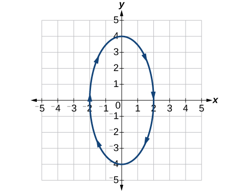
16. \(\left\{ \begin{array}{l} {x(t) = 4\text{sin}\; t} \\ {y(t) = 2\cos\; t} \end{array} \right.\)
17. \(\left\{ \begin{array}{l} {x(t) = 2\text{sin}\; t} \\ {y(t) = 4\text{cos}\; t} \end{array} \right.\)
Solution (click to reveal)
18. \(\left\{ \begin{array}{l} {x(t) = 3\cos^{2}t} \\ {y(t) = -3\sin\; t} \end{array} \right.\)
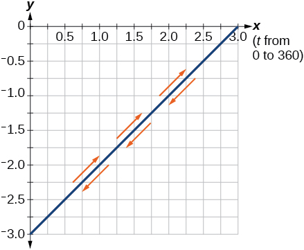
19. \(\left\{ \begin{array}{l} {x(t) = 3\cos^{2}t} \\ {y(t) = -3\sin^{2}t} \end{array} \right.\)
Solution (click to reveal)
20. \(\left\{ \begin{array}{l} {x(t) = \sec\; t} \\ {y(t) = \tan\; t} \end{array} \right.\)
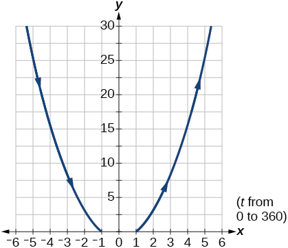
21. \(\left\{ \begin{array}{l} {x(t) = \sec\; t} \\ {y(t) = \tan^{2}t} \end{array} \right.\)
Solution (click to reveal)
22. \(\left\{ \begin{array}{l} {x(t) = \frac{1}{e^{2t}}} \\ {y(t) = e^{- \; t}} \end{array} \right.\)
For the following exercises, graph the equation and include the orientation. Then, write the Cartesian equation.
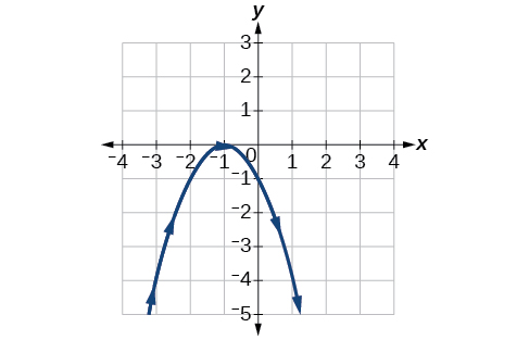
23. \(\left\{ \begin{array}{l} {x(t) = t - 1} \\ {y(t) = - t^{2}} \end{array} \right.\)
Solution (click to reveal)
24. \(\left\{ \begin{array}{l} {x(t) = t^{3}} \\ {y(t) = t + 3} \end{array} \right.\)
25. \(\left\{ \begin{array}{l} {x(t) = 2\cos\; t} \\ {y(t) = - \sin\; t} \end{array} \right.\)
Solution (click to reveal)
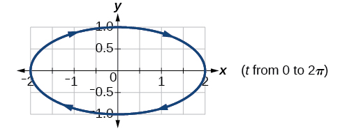
26. \(\left\{ \begin{array}{l} {x(t) = 7\cos\; t} \\ {y(t) = 7\sin\; t} \end{array} \right.\)
27. \(\left\{ \begin{array}{l} {x(t) = e^{2t}} \\ {y(t) = - e^{\; t}} \end{array} \right.\)
Solution (click to reveal)
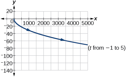
For the following exercises, graph the equation and include the orientation.
28. \(x = t^{2},\; y\; = \; 3t,\; 0 \leq t \leq 5\)
29. \(x = 2t,\; y = \mspace{9mu} t^{2},\; - 5 \leq t \leq 5\)
Solution (click to reveal)
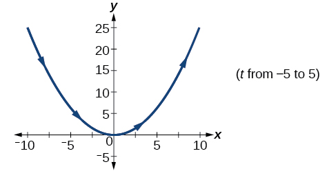
30. \(x = t,\) \(y = \sqrt{25 - t^{2}},\) \(0 < t \leq 5\)
31. \(x(t) = - t,y(t) = \sqrt{t},\) \(t \geq 0\)
Solution (click to reveal)
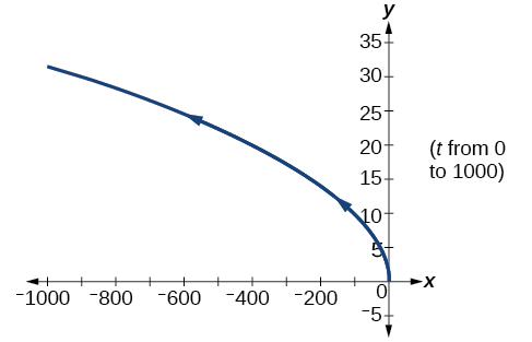
32. \(x = - 2\cos\; t,\) \(y = 6\;\sin\; t,\) \(0 \leq t \leq \pi\)
33. \(x = - \sec\; t,\) \(y = \tan\; t,\) \(- \frac{\pi}{2} < t < \frac{\pi}{2}\)
Solution (click to reveal)
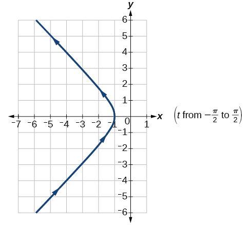
For the following exercises, use the parametric equations for integers a and \(b\):
\[\begin{array}{l} {x(t) = a\cos((a + b)t)} \\ {y(t) = a\cos((a - b)t)} \end{array}\]
34. Graph on the domain \(\left\lbrack {- \pi,0} \right\rbrack,\) where \(a = 2\) and \(b = 1,\) and include the orientation.
35. Graph on the domain \(\left\lbrack {- \pi,0} \right\rbrack,\) where \(a = 3\) and \(b = 2\), and include the orientation.
Solution (click to reveal)
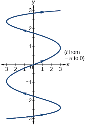
36. Graph on the domain \(\left\lbrack {- \pi,0} \right\rbrack,\) where \(a = 4\) and \(b = 3\), and include the orientation.
37. Graph on the domain \(\left\lbrack {- \pi,0} \right\rbrack,\) where \(a = 5\) and \(b = 4\), and include the orientation.
Solution (click to reveal)
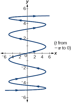
38. If \(a\) is 1 more than \(b,\) describe the effect the values of \(a\) and \(b\) have on the graph of the parametric equations.
39. Describe the graph if \(a = 100\) and \(b = 99.\)
Solution (click to reveal)
There will be 100 back-and-forth motions.
40. What happens if \(b\) is 1 more than \(a?\) Describe the graph.
41. If the parametric equations \(x(t) = t^{2}\) and \(y(t) = 6 - 3t\) have the graph of a horizontal parabola opening to the right, what would change the direction of the curve?
Solution (click to reveal)
Take the opposite of the \(x(t)\) equation.
For the following exercises, describe the graph of the set of parametric equations.
42. \(x(t) = - t^{2}\) and \(y(t)\) is linear
43. \(y(t) = t^{2}\) and \(x(t)\) is linear
Solution (click to reveal)
The parabola opens up.
44. \(y(t) = - t^{2}\) and \(x(t)\) is linear
45. Write the parametric equations of a circle with center \(\left( {0,0} \right),\) radius 5, and a counterclockwise orientation.
Solution (click to reveal)
\(\left\{ \begin{array}{l} {x(t) = 5\cos t} \\ {y(t) = 5\sin t} \end{array} \right.\)
46. Write the parametric equations of an ellipse with center \(\left( {0,0} \right),\) major axis of length 10, minor axis of length 6, and a counterclockwise orientation.
For the following exercises, use a graphing utility to graph on the window \(\left\lbrack {- 3,3} \right\rbrack\) by \(\left\lbrack {- 3,3} \right\rbrack\) on the domain \(\lbrack 0,2\pi)\) for the following values of \(a\) and \(b\), and include the orientation.
\[\left\{ \begin{array}{l} {x(t) = \sin(at)} \\ {y(t) = \sin(bt)} \end{array} \right.\]
47. \(a = 1,b = 2\)
Solution (click to reveal)
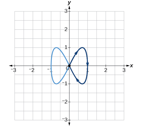
48. \(a = 2,b = 1\)
49. \(a = 3,b = 3\)
Solution (click to reveal)
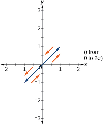
50. \(a = 5,b = 5\)
51. \(a = 2,b = 5\)
Solution (click to reveal)
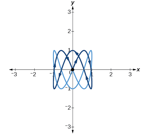
52. \(a = 5,b = 2\)
Technology
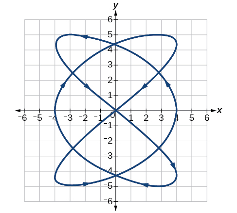
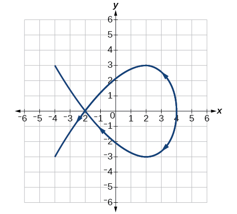
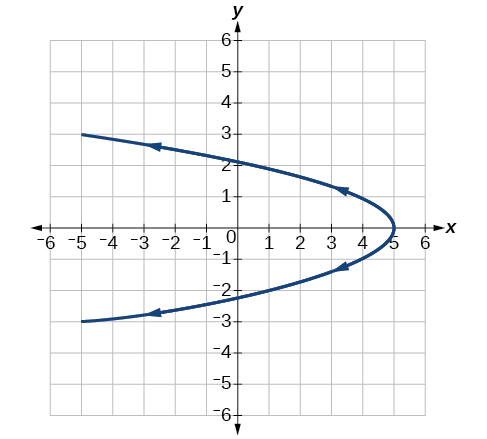
For the following exercises, look at the graphs that were created by parametric equations of the form \(\left\{ \begin{array}{l} {x(t) = a\text{cos}(bt)} \\ {y(t) = c\text{sin}(dt)} \end{array}. \right.\) Use the parametric mode on the graphing calculator to find the values of \(a,b,c,\) and \(d\) to achieve each graph.
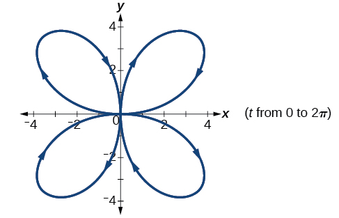
53.
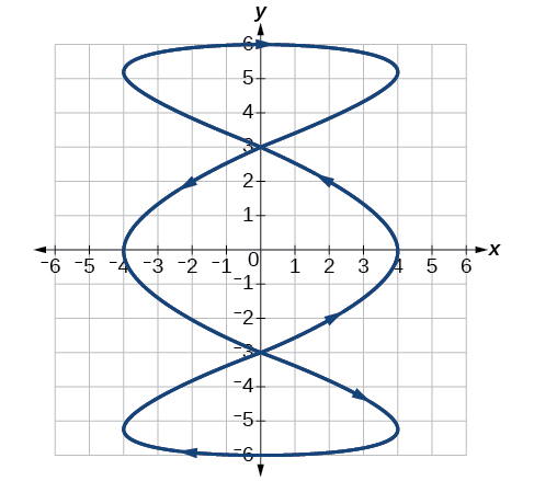
Solution (click to reveal)
\(a = 4,\) \(b = 3,\) \(c = 6,\) \(d = 1\)
54.
55.
Solution (click to reveal)
\(a = 4,\) \(b = 2,\) \(c = 3,\) \(d = 3\)
56.
For the following exercises, use a graphing utility to graph the given parametric equations.
1. \(\left\{ \begin{array}{l} {x(t) = \cos t - 1} \\ {y(t) = \sin t + t} \end{array} \right.\)
2. \(\left\{ \begin{array}{l} {x(t) = \cos t + t} \\ {y(t) = \sin t - 1} \end{array} \right.\)
3. \(\left\{ \begin{array}{l} {x(t) = t - \sin t} \\ {y(t) = \cos t - 1} \end{array} \right.\)
57. Graph all three sets of parametric equations on the domain \(\lbrack 0,\) \(2\pi\rbrack.\)
Solution (click to reveal)
![Graph of the parametric equations x(t) = cos(t) minus 1 and y(t) = sin(t) + t on the domain [0, 2 pi]. The curve starts at the origin and rises to the left in a cusp-like shape, reaching about (negative 2, 4) before curving back down toward (0, 2 pi), resembling a sideways teardrop opening to the left.](../images/CNX_Precalc_Figure_08_07_243.jpg)
![Graph of parametric equations on the domain [0, 2pi]. The curve starts near (1, -1), dips to a minimum y-value around -2 near x = 3, then rises back up to end near (2pi + 1, -1). Directional arrows show the curve moving left to right.](../images/CNX_Precalc_Figure_08_07_244.jpg)
![Graph of parametric equations on the domain [0, 2pi]. The curve starts at the origin, dips down to a minimum y-value of about -2 near x = pi, then returns to approximately (2pi, 0). Directional arrows show the curve moving left to right.](../images/CNX_Precalc_Figure_08_07_245.jpg)
58. Graph all three sets of parametric equations on the domain \(\left\lbrack {0,4\pi} \right\rbrack.\)
59. Graph all three sets of parametric equations on the domain \(\left\lbrack {- 4\pi,6\pi} \right\rbrack.\)
Solution (click to reveal)
![Graph of parametric equations on the domain [-4pi, 6pi]. The curve oscillates horizontally between roughly x = -2 and x = 0 while steadily increasing in y, creeping upward along the y-axis from about y = -10 to y = 20.](../images/CNX_Precalc_Figure_08_07_249.jpg)
![Graph of parametric equations on the domain [-4pi, 6pi]. The curve oscillates vertically with peaks near y = 0 and troughs near y = -2, while steadily advancing to the right along the x-axis from about x = -10 to x = 20.](../images/CNX_Precalc_Figure_08_07_250.jpg)
![Graph of the parametric equations x(t) = t minus sin(t) and y(t) = cos(t) minus 1 on the domain [negative 4 pi, 6 pi]. The curve forms a series of inverted cusps (an inverted cycloid), oscillating between y = 0 and y = negative 2, with five full arches spread across x values from about negative 10 to 20.](../images/CNX_Precalc_Figure_08_07_251.jpg)
60. The graph of each set of parametric equations appears to “creep” along one of the axes. What controls which axis the graph creeps along?
61. Explain the effect on the graph of the parametric equation when we switched \(\sin\; t\) and \(\cos\; t\).
Solution (click to reveal)
The \(y\)-intercept changes.
62. Explain the effect on the graph of the parametric equation when we changed the domain.
Extensions
63. An object is thrown in the air with vertical velocity of 20 ft/s and horizontal velocity of 15 ft/s. The object’s height can be described by the equation \(y(t) = - 16t^{2} + 20t\), while the object moves horizontally with constant velocity 15 ft/s. Write parametric equations for the object’s position, and then eliminate time to write height as a function of horizontal position.
Solution (click to reveal)
\(y(x) = - 16\left( \frac{x}{15} \right)^{2} + 20\left( \frac{x}{15} \right)\)
64. A skateboarder riding on a level surface at a constant speed of 9 ft/s throws a ball in the air, the height of which can be described by the equation \(y(t) = - 16t^{2} + 10t + 5.\) Write parametric equations for the ball’s position, and then eliminate time to write height as a function of horizontal position.
For the following exercises, use this scenario: A dart is thrown upward with an initial velocity of 64 ft/s at an angle of elevation of 52°. Consider the position of the dart at any time \(t.\) Neglect air resistance.
65. Find parametric equations that model the problem situation.
Solution (click to reveal)
\(\left\{ \begin{array}{l} {x(t) = 64t\cos\left( {52{^\circ}} \right)} \\ {y(t) = - 16t^{2} + 64t\sin\left( {52{^\circ}} \right)} \end{array} \right.\)
66. Find all possible values of \(x\) that represent the situation.
67. When will the dart hit the ground?
Solution (click to reveal)
approximately 3.2 seconds
68. Find the maximum height of the dart.
69. At what time will the dart reach maximum height?
Solution (click to reveal)
1.6 seconds
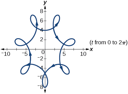
For the following exercises, look at the graphs of each of the four parametric equations. Although they look unusual and beautiful, they are so common that they have names, as indicated in each exercise. Use a graphing utility to graph each on the indicated domain.
70. An epicycloid: \(\left\{ \begin{array}{l} {x(t) = 14\cos\; t - \cos(14t)} \\ {y(t) = 14\sin\; t + \sin(14t)} \end{array} \right.\) on the domain \(\lbrack 0,2\pi\rbrack\).
71. A hypocycloid: \(\left\{ \begin{array}{l} {x(t) = 6\sin\; t + 2\sin(6t)} \\ {y(t) = 6\cos\; t - 2\cos(6t)} \end{array} \right.\) on the domain \(\lbrack 0,2\pi\rbrack\).
Solution (click to reveal)
72. A hypotrochoid: \(\left\{ \begin{array}{l} {x(t) = 2\sin\; t + 5\cos(6t)} \\ {y(t) = 5\cos\; t - 2\sin(6t)} \end{array} \right.\) on the domain \(\lbrack 0,2\pi\rbrack\).
73. A rose: \(\left\{ \begin{array}{l} {x(t) = 5\sin(2t)\sin t} \\ {y(t) = 5\sin(2t)\cos t} \end{array} \right.\) on the domain \(\lbrack 0,2\pi\rbrack\).
Solution (click to reveal)