Chapter Review

Key Terms

absolute maximum — the greatest value of a function over an interval

absolute minimum — the lowest value of a function over an interval

average rate of change — the difference in the output values of a function found for two values of the input divided by the difference between the inputs

composite function — the new function formed by function composition, when the output of one function is used as the input of another

decreasing function — a function is decreasing in some open interval if \(f(b) < f(a)\) for any two input values \(a\) and \(b\) in the given interval where \(b > a\)

dependent variable — an output variable

domain — the set of all possible input values for a relation

even function — a function whose graph is unchanged by horizontal reflection, \(f(x) = f( - x),\) and is symmetric about the \(y\text{-}\) axis

function — a relation in which each input value yields a unique output value

horizontal compression — a transformation that compresses a function’s graph horizontally, by multiplying the input by a constant \(b > 1\)

horizontal line test — a method of testing whether a function is one-to-one by determining whether any horizontal line intersects the graph more than once

horizontal reflection — a transformation that reflects a function’s graph across the \(y\)-axis by multiplying the input by \(-1\)

horizontal shift — a transformation that shifts a function’s graph left or right by adding a positive or negative constant to the input

horizontal stretch — a transformation that stretches a function’s graph horizontally by multiplying the input by a constant \(0 < b < 1\)

increasing function — a function is increasing in some open interval if \(f(b) > f(a)\) for any two input values \(a\) and \(b\) in the given interval where \(b > a\)

independent variable — an input variable

input — each object or value in a domain that relates to another object or value by a relationship known as a function

interval notation — a method of describing a set that includes all numbers between a lower limit and an upper limit; the lower and upper values are listed between brackets or parentheses, a square bracket indicating inclusion in the set, and a parenthesis indicating exclusion

inverse function — for any one-to-one function \(f(x),\) the inverse is a function \(f^{- 1}(x)\) such that \(f^{- 1}\left( {f(x)} \right) = x\) for all \(x\) in the domain of \(f;\) this also implies that \(f\left( {f^{- 1}(x)} \right) = x\) for all \(x\) in the domain of \(f^{- 1}\)

local extrema — collectively, all of a function’s local maxima and minima

local maximum — a value of the input where a function changes from increasing to decreasing as the input value increases.

local minimum — a value of the input where a function changes from decreasing to increasing as the input value increases.

odd function — a function whose graph is unchanged by combined horizontal and vertical reflection, \(f(x) = - f( - x),\) and is symmetric about the origin

one-to-one function — a function for which each value of the output is associated with a unique input value

output — each object or value in the range that is produced when an input value is entered into a function

piecewise function — a function in which more than one formula is used to define the output

range — the set of output values that result from the input values in a relation

rate of change — the change of an output quantity relative to the change of the input quantity

relation — a set of ordered pairs

set-builder notation — a method of describing a set by a rule that all of its members obey; it takes the form \(\left\{ x \middle| \mspace{9mu}\text{statement~about~}x \right\}\)

vertical compression — a function transformation that compresses the function’s graph vertically by multiplying the output by a constant \(0 < a < 1\)

vertical line test — a method of testing whether a graph represents a function by determining whether a vertical line intersects the graph no more than once

vertical reflection — a transformation that reflects a function’s graph across the \(x\)-axis by multiplying the output by \(-1\)

vertical shift — a transformation that shifts a function’s graph up or down by adding a positive or negative constant to the output

vertical stretch — a transformation that stretches a function’s graph vertically by multiplying the output by a constant \(a > 1\)

Key Equations

Constant function	\(f(x) = c,\) where \(c\) is a constant
Identity function	\(f(x) = x\)
Absolute value function	\(f(x) = |x|\)
Quadratic function	\(f(x) = x^{2}\)
Cubic function	\(f(x) = x^{3}\)
Reciprocal function	\(f(x) = \frac{1}{x}\)
Reciprocal squared function	\(f(x) = \frac{1}{x^{2}}\)
Square root function	\(f(x) = \sqrt{x}\)
Cube root function	\(f(x) = \sqrt[3]{x}\)

Average rate of change

\(\frac{\Delta y}{\Delta x} = \frac{f\left( x_{2} \right) - f\left( x_{1} \right)}{x_{2} - x_{1}}\)

Composite function

\(\left( {f \circ g} \right)(x) = f\left( {g(x)} \right)\)

Vertical shift	\(g(x) = f(x) + k\) (up for \(k > 0\) )
Horizontal shift	\(g(x) = f(x - h)\) (right for \(h > 0\) )
Vertical reflection	\(g(x) = - f(x)\)
Horizontal reflection	\(g(x) = f( - x)\)
Vertical stretch	\(g(x) = af(x)\) ( \(a > 0\) )
Vertical compression	\(g(x) = af(x)\) \((0 < a < 1)\)
Horizontal stretch	\(g(x) = f(bx)\) \((0 < b < 1)\)
Horizontal compression.	\(g(x) = f(bx)\) ( \(b > 1\) )

Key Concepts

3.1 Functions and Function Notation

• A relation is a set of ordered pairs. A function is a specific type of relation in which each domain value, or input, leads to exactly one range value, or output. See Example 1 and Example 2.
• Function notation is a shorthand method for relating the input to the output in the form \(y = f(x).\) See Example 3 and Example 4.
• In tabular form, a function can be represented by rows or columns that relate to input and output values. See Example 5.
• To evaluate a function, we determine an output value for a corresponding input value. Algebraic forms of a function can be evaluated by replacing the input variable with a given value. See Example 6 and Example 7.
• To solve for a specific function value, we determine the input values that yield the specific output value. See Example 8.
• An algebraic form of a function can be written from an equation. See Example 9 and Example 10.
• Input and output values of a function can be identified from a table. See Example 11.
• Relating input values to output values on a graph is another way to evaluate a function. See Example 12.
• A function is one-to-one if each output value corresponds to only one input value. See Example 13.
• A graph represents a function if any vertical line drawn on the graph intersects the graph at no more than one point. See Example 14.
• The graph of a one-to-one function passes the horizontal line test. See Example 15.

3.2 Domain and Range

• The domain of a function includes all real input values that would not cause us to attempt an undefined mathematical operation, such as dividing by zero or taking the square root of a negative number.
• The domain of a function can be determined by listing the input values of a set of ordered pairs. See Example 1.
• The domain of a function can also be determined by identifying the input values of a function written as an equation. See Example 2, Example 3, and Example 4.
• Interval values represented on a number line can be described using inequality notation, set-builder notation, and interval notation. See Example 5.
• For many functions, the domain and range can be determined from a graph. See Example 6 and Example 7.
• An understanding of toolkit functions can be used to find the domain and range of related functions. See Example 8, Example 9, and Example 10.
• A piecewise function is described by more than one formula. See Example 11 and Example 12.
• A piecewise function can be graphed using each algebraic formula on its assigned subdomain. See Example 13.

3.3 Rates of Change and Behavior of Graphs

• A rate of change relates a change in an output quantity to a change in an input quantity. The average rate of change is determined using only the beginning and ending data. See Example 1.
• Identifying points that mark the interval on a graph can be used to find the average rate of change. See Example 2.
• Comparing pairs of input and output values in a table can also be used to find the average rate of change. See Example 3.
• An average rate of change can also be computed by determining the function values at the endpoints of an interval described by a formula. See Example 4 and Example 5.
• The average rate of change can sometimes be determined as an expression. See Example 6.
• A function is increasing where its rate of change is positive and decreasing where its rate of change is negative. See Example 7.
• A local maximum is where a function changes from increasing to decreasing and has an output value larger (more positive or less negative) than output values at neighboring input values.
• A local minimum is where the function changes from decreasing to increasing (as the input increases) and has an output value smaller (more negative or less positive) than output values at neighboring input values.
• Minima and maxima are also called extrema.
• We can find local extrema from a graph. See Example 8 and Example 9.
• The highest and lowest points on a graph indicate the maxima and minima. See Example 10.

3.4 Composition of Functions

• We can perform algebraic operations on functions. See Example 1.
• When functions are composed, the output of the first (inner) function becomes the input of the second (outer) function.
• The function produced by composing two functions is a composite function. See Example 2 and Example 3.
• The order of function composition must be considered when interpreting the meaning of composite functions. See Example 4.
• A composite function can be evaluated by evaluating the inner function using the given input value and then evaluating the outer function taking as its input the output of the inner function.
• A composite function can be evaluated from a table. See Example 5.
• A composite function can be evaluated from a graph. See Example 6.
• A composite function can be evaluated from a formula. See Example 7.
• The domain of a composite function consists of those inputs in the domain of the inner function that correspond to outputs of the inner function that are in the domain of the outer function. See Example 8 and Example 9.
• Just as functions can be combined to form a composite function, composite functions can be decomposed into simpler functions.
• Functions can often be decomposed in more than one way. See Example 10.

3.5 Transformation of Functions

• A function can be shifted vertically by adding a constant to the output. See Example 1 and Example 2.
• A function can be shifted horizontally by adding a constant to the input. See Example 3, Example 4, and Example 5.
• Relating the shift to the context of a problem makes it possible to compare and interpret vertical and horizontal shifts. See Example 6.
• Vertical and horizontal shifts are often combined. See Example 7 and Example 8.
• A vertical reflection reflects a graph about the \(x\text{-}\) axis. A graph can be reflected vertically by multiplying the output by –1.
• A horizontal reflection reflects a graph about the \(y\text{-}\) axis. A graph can be reflected horizontally by multiplying the input by –1.
• A graph can be reflected both vertically and horizontally. The order in which the reflections are applied does not affect the final graph. See Example 9.
• A function presented in tabular form can also be reflected by multiplying the values in the input and output rows or columns accordingly. See Example 10.
• A function presented as an equation can be reflected by applying transformations one at a time. See Example 11.
• Even functions are symmetric about the \(y\text{-}\) axis, whereas odd functions are symmetric about the origin.
• Even functions satisfy the condition \(f(x) = f( - x).\)
• Odd functions satisfy the condition \(f(x) = - f( - x).\)
• A function can be odd, even, or neither. See Example 12.
• A function can be compressed or stretched vertically by multiplying the output by a constant. See Example 13, Example 14, and Example 15.
• A function can be compressed or stretched horizontally by multiplying the input by a constant. See Example 16, Example 17, and Example 18.
• The order in which different transformations are applied does affect the final function. Both vertical and horizontal transformations must be applied in the order given. However, a vertical transformation may be combined with a horizontal transformation in any order. See Example 19 and Example 20.

3.6 Absolute Value Functions

• Applied problems, such as ranges of possible values, can also be solved using the absolute value function. See Example 1.
• The graph of the absolute value function resembles a letter V. It has a corner point at which the graph changes direction. See Example 2.
• In an absolute value equation, an unknown variable is the input of an absolute value function.
• If the absolute value of an expression is set equal to a positive number, expect two solutions for the unknown variable. See Example 3.

3.7 Inverse Functions

• If \(g(x)\) is the inverse of \(f(x),\) then \(g(f(x)) = f(g(x)) = x.\) See Example 1, Example 2, and Example 3.
• Only some of the toolkit functions have an inverse. See Example 4.
• For a function to have an inverse, it must be one-to-one (pass the horizontal line test).
• A function that is not one-to-one over its entire domain may be one-to-one on part of its domain.
• For a tabular function, exchange the input and output rows to obtain the inverse. See Example 5.
• The inverse of a function can be determined at specific points on its graph. See Example 6.
• To find the inverse of a formula, solve the equation \(y = f(x)\) for \(x\) as a function of \(y.\) Then exchange the labels \(x\) and \(y.\) See Example 7, Example 8, and Example 9.
• The graph of an inverse function is the reflection of the graph of the original function across the line \(y = x.\) See Example 10.

Chapter Review Exercises

Functions and Function Notation

For the following exercises, determine whether the relation is a function.

1. \(\left\{ {(a,b),(c,d),(e,d)} \right\}\)

Solution (click to reveal)

function

2. \(\left\{ {(5,2),(6,1),(6,2),(4,8)} \right\}\)

3. \(y^{2} + 4 = x,\) for \(x\) the independent variable and \(y\) the dependent variable

Solution (click to reveal)

not a function

4. Is the graph in Figure 13 a function?

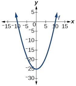
Figure 13

For the following exercises, evaluate \(\mspace{9mu}\mspace{9mu} f( - 3);\mspace{9mu}\mspace{9mu} f(2);\mspace{9mu}\mspace{9mu}\mspace{9mu} f( - a);\mspace{9mu}\mspace{9mu}\mspace{9mu} - f(a);\mspace{9mu}\mspace{9mu}\mspace{9mu} f(a + h).\)

5. \(f(x) = - 2x^{2} + 3x\)

Solution (click to reveal)

\(f( - 3) = - 27;\) \(f(2) = - 2;\) \(f( - a) = - 2a^{2} - 3a;\)
\(- f(a) = 2a^{2} - 3a;\) \(f(a + h) = - 2a^{2} + 3a - 4ah + 3h - 2h^{2}\)

6. \(f(x) = 2\left| {3x - 1} \right|\)

For the following exercises, determine whether the functions are one-to-one.

7. \(f(x) = - 3x + 5\)

Solution (click to reveal)

one-to-one

8. \(f(x) = \left| {x - 3} \right|\)

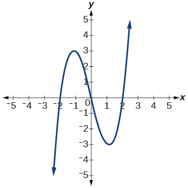
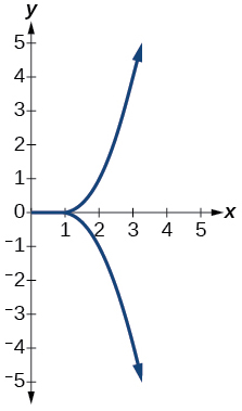
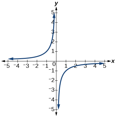
For the following exercises, use the vertical line test to determine if the relation whose graph is provided is a function.

9.

Solution (click to reveal)

function

10.

11.

Solution (click to reveal)

function

For the following exercises, graph the functions.

12. \(f(x) = \left| {x + 1} \right|\)

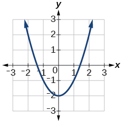
13. \(f(x) = x^{2} - 2\)

Solution (click to reveal)

For the following exercises, use Figure 14 to approximate the values.

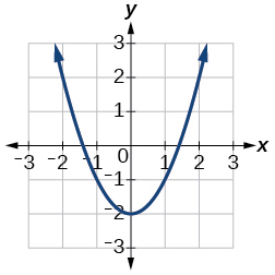
Figure 14

14. \(f(2)\)

15. \(f(-2)\)

Solution (click to reveal)

\(2\)

16. If \(f(x) = -2,\) then solve for \(x.\)

17. If \(f(x) = 1,\) then solve for \(x.\)

Solution (click to reveal)

\(x = - 1.8\) or \(\text{or~}x = 1.8\)

For the following exercises, use the function \(h(t) = - 16t^{2} + 80t\) to find the values in simplest form.

18. \(\frac{h(2) - h(1)}{2 - 1}\)

19. \(\frac{h(a) - h(1)}{a - 1}\)

Solution (click to reveal)

\(\frac{- 64 + 80a - 16a^{2}}{- 1 + a} = - 16a + 64\)

Domain and Range

For the following exercises, find the domain of each function, expressing answers using interval notation.

20. \(f(x) = \frac{2}{3x + 2}\)

21. \(f(x) = \frac{x - 3}{x^{2} - 4x - 12}\)

Solution (click to reveal)

\(\left( {- \infty, - 2} \right) \cup \left( {- 2,6} \right) \cup \left( {6,\infty} \right)\)

22. \(f(x) = \frac{\sqrt{x - 6}}{\sqrt{x - 4}}\)

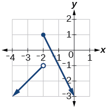
23. Graph this piecewise function: \(f(x) = \left\{ \begin{array}{l} {x + 1\mspace{9mu}\text{~~~~~~~}x < - 2} \\ {- 2x - 3\mspace{9mu}\text{~~}x \geq - 2} \end{array} \right.\)

Solution (click to reveal)

Rates of Change and Behavior of Graphs

For the following exercises, find the average rate of change of the functions from \(x = 1\mspace{9mu}\text{to~}x = 2.\)

24. \(f(x) = 4x - 3\)

25. \(f(x) = 10x^{2} + x\)

Solution (click to reveal)

\(31\)

26. \(f(x) = - \frac{2}{x^{2}}\)

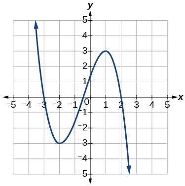
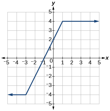
For the following exercises, use the graphs to determine the intervals on which the functions are increasing, decreasing, or constant.

27.

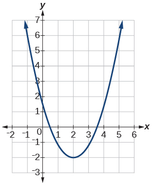
Solution (click to reveal)

increasing \(\left( {2,\infty} \right);\) decreasing \(( - \infty,2)\)

28.

29.

Solution (click to reveal)

increasing \(\left( {- 3,1} \right);\) constant \(( - \infty, - 3) \cup \left( {1,\infty} \right)\)

30. Find the local minimum of the function graphed in Exercise 93.

31. Find the local extrema for the function graphed in Exercise 94.

Solution (click to reveal)

local minimum \(\left( {- 2, - 3} \right);\) local maximum \(\left( {1,3} \right)\)

32. For the graph in Figure 15, the domain of the function is \(\left\lbrack {- 3,3} \right\rbrack.\) The range is \(\left\lbrack {- 10,10} \right\rbrack.\) Find the absolute minimum of the function on this interval.

33. Find the absolute maximum of the function graphed in Figure 15.

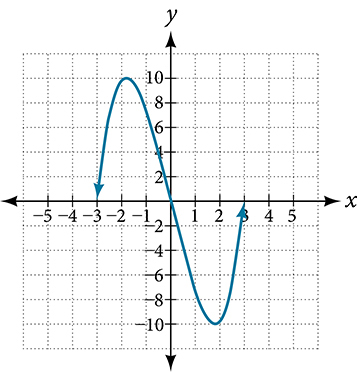
Figure 15

Solution (click to reveal)

\(\left( {- 1.8,10} \right)\)

Composition of Functions

For the following exercises, find \((f \circ g)(x)\) and \((g \circ f)(x)\) for each pair of functions.

34. \(f(x) = 4 - x,\mspace{9mu} g(x) = - 4x\)

35. \(f(x) = 3x + 2,\mspace{9mu} g(x) = 5 - 6x\)

Solution (click to reveal)

\(\left( {f \circ g} \right)(x) = 17 - 18x;\mspace{9mu}\left( {g \circ f} \right)(x) = - 7 - 18x\)

36. \(f(x) = x^{2} + 2x,\mspace{9mu} g(x) = 5x + 1\)

37. \(f(x) = \sqrt{x + 2},\mspace{9mu} g(x) = \frac{1}{x}\)

Solution (click to reveal)

\(\left( {f \circ g} \right)(x) = \sqrt{\frac{1}{x} + 2};\mspace{9mu}\left( {g \circ f} \right)(x) = \frac{1}{\sqrt{x + 2}}\)

38. \(f(x) = \frac{x + 3}{2},\mspace{9mu} g(x) = \sqrt{1 - x}\)

For the following exercises, find \(\left( {f \circ g} \right)\) and the domain for \(\left( {f \circ g} \right)(x)\) for each pair of functions.

39. \(f(x) = \frac{x + 1}{x + 4},\mspace{9mu} g(x) = \frac{1}{x}\)

Solution (click to reveal)

\((f \circ g)(x) = \frac{1 + x}{1 + 4x},~x \neq 0,~x \neq - \frac{1}{4}\)

40. \(f(x) = \frac{1}{x + 3},\mspace{9mu} g(x) = \frac{1}{x - 9}\)

41. \(f(x) = \frac{1}{x},\mspace{9mu} g(x) = \sqrt{x}\)

Solution (click to reveal)

\(\left( {f \circ g} \right)(x) = \frac{1}{\sqrt{x}},\mspace{9mu} x > 0\)

42. \(f(x) = \frac{1}{x^{2} - 1},\mspace{9mu} g(x) = \sqrt{x + 1}\)

For the following exercises, express each function \(H\) as a composition of two functions \(f\) and \(g\) where \(H(x) = (f \circ g)(x).\)

43. \(H(x) = \sqrt{\frac{2x - 1}{3x + 4}}\)

Solution (click to reveal)

sample: \(g(x) = \frac{2x - 1}{3x + 4};\mspace{9mu} f(x) = \sqrt{x}\)

44. \(H(x) = \frac{1}{{(3x^{2} - 4)}^{- 3}}\)

Transformation of Functions

For the following exercises, sketch a graph of the given function.

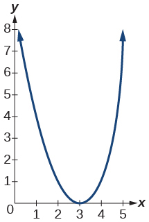
45. \(f(x) = {(x - 3)}^{2}\)

Solution (click to reveal)

46. \(f(x) = {(x + 4)}^{3}\)

47. \(f(x) = \sqrt{x} + 5\)

Solution (click to reveal)

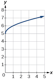
48. \(f(x) = - x^{3}\)

49. \(f(x) = \sqrt[3]{- x}\)

Solution (click to reveal)

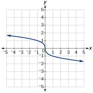
50. \(f(x) = 5\sqrt{- x} - 4\)

51. \(f(x) = 4\left\lbrack {\left| {x - 2} \right| - 6} \right\rbrack\)

Solution (click to reveal)

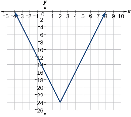
52. \(f(x) = - {(x + 2)}^{2} - 1\)

For the following exercises, sketch the graph of the function \(g\) if the graph of the function \(f\) is shown in Figure 16.

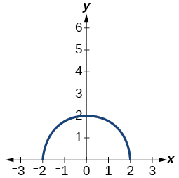
Figure 16

53. \(g(x) = f(x - 1)\)

Solution (click to reveal)

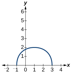
54. \(g(x) = 3f(x)\)

For the following exercises, write the equation for the standard function represented by each of the graphs below.

55.

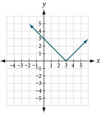
Solution (click to reveal)

\(f(x) = \left| {x - 3} \right|\)

56.

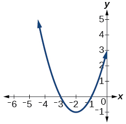
For the following exercises, determine whether each function below is even, odd, or neither.

57. \(f(x) = 3x^{4}\)

Solution (click to reveal)

even

58. \(g(x) = \sqrt{x}\)

59. \(h(x) = \frac{1}{x} + 3x\)

Solution (click to reveal)

odd

For the following exercises, analyze the graph and determine whether the graphed function is even, odd, or neither.

60.

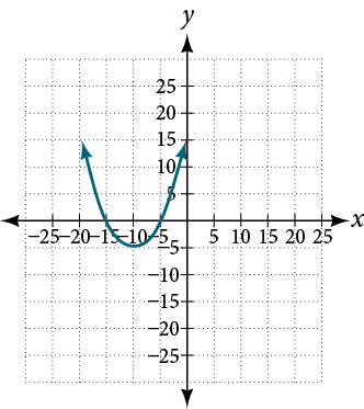
61.

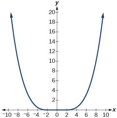
Solution (click to reveal)

even

62.

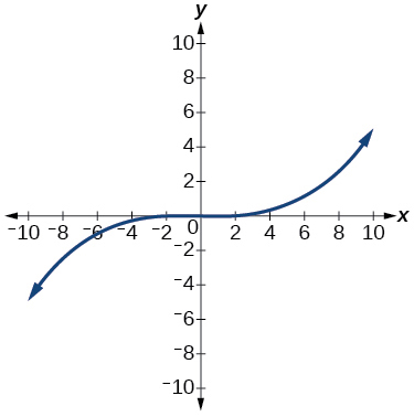
Absolute Value Functions

For the following exercises, write an equation for the transformation of \(f(x) = |x|.\)

63.

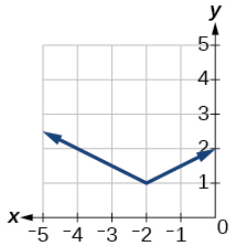
Solution (click to reveal)

\(f(x) = \frac{1}{2}\left| {x + 2} \right| + 1\)

64.

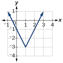
65.

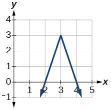
Solution (click to reveal)

\(f(x) = - 3\left| {x - 3} \right| + 3\)

For the following exercises, graph the absolute value function.

66. \(f(x) = \left| {x - 5} \right|\)

67. \(f(x) = - \left| {x - 3} \right|\)

Solution (click to reveal)

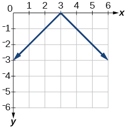
68. \(f(x) = \left| {2x - 4} \right|\)

Inverse Functions

For the following exercises, find \(f^{- 1}(x)\) for each function.

69. \(f(x) = 9 + 10x\)

Solution (click to reveal)

\({f^{- 1}(x)} = \frac{x - 9}{10}\)

70. \(f(x) = \frac{x}{x + 2}\)

For the following exercise, find a domain on which the function \(f\) is one-to-one and non-decreasing. Write the domain in interval notation. Then find the inverse of \(f\) restricted to that domain.

71. \(f(x) = x^{2} + 1\)

Solution (click to reveal)

\({f^{- 1}(x)} = \sqrt{x - 1}\)

72. Given \(f(x) = x^{3} - 5\) and \(g(x) = \sqrt[3]{x + 5}:\)

ⓐ Find \(~f(g(x))\) and \(g(f(x)).\)

ⓑ What does the answer tell us about the relationship between \(f(x)\) and \(g(x)?\)

For the following exercises, use a graphing utility to determine whether each function is one-to-one.

73. \(f(x) = \frac{1}{x}\)

Solution (click to reveal)

The function is one-to-one.

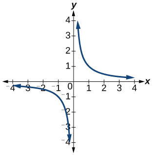
74. \(f(x) = - 3x^{2} + x\)

75. If \(f(5) = 2,\) find \(f^{- 1}(2).\)

Solution (click to reveal)

\(5\)

76. If \(f(1) = 4,\) find \(f^{- 1}(4).\)

Practice Test

For the following exercises, determine whether each of the following relations is a function.

1. \(y = 2x + 8\)

Solution (click to reveal)

The relation is a function.

2. \(\left\{ {(2,1),(3,2),( - 1,1),(0, - 2)} \right\}\)

For the following exercises, evaluate the function \(f(x) = - 3x^{2} + 2x\) at the given input.

3. \(f(-2)\)

Solution (click to reveal)

−16

4. \(f(a)\)

5. Show that the function \(f(x) = - 2{(x - 1)}^{2} + 3\) is not one-to-one.

Solution (click to reveal)

The graph is a parabola and the graph fails the horizontal line test.

6. Write the domain of the function \(f(x) = \sqrt{3 - x}\) in interval notation.

7. Given \(f(x) = 2x^{2} - 5x,\) find \(f(a + 1) - f(1)\) in simplest form.

Solution (click to reveal)

\(2a^{2} - a\)

8. Graph the function \(f(x) = \left\{ \begin{matrix} {x + 1\mspace{9mu}\text{~~if}} & {- 2 < x < 3} \\ {\mspace{9mu}\text{~~} - x\mspace{9mu}\text{~~~if~~}} & {x \geq 3} \end{matrix} \right.\)

9. Find the average rate of change of the function \(f(x) = 3 - 2x^{2} + x\) by finding \(\frac{f(b) - f(a)}{b - a}\) in simplest form.

Solution (click to reveal)

\(- 2(a + b) + 1\)

For the following exercises, use the functions \(f(x) = 3 - 2x^{2} + x\mspace{9mu}\text{and~}g(x) = \sqrt{x}\) to find the composite functions.

10. \(\left( {g \circ f} \right)(x)\)

11. \(\left( {g \circ f} \right)(1)\)

Solution (click to reveal)

\(\sqrt{2}\)

12. Express \(H(x) = \sqrt[3]{5x^{2} - 3x}\) as a composition of two functions, \(f\) and \(g,\) where \(\left( {f \circ g} \right)(x) = H(x).\)

For the following exercises, graph the functions by translating, stretching, and/or compressing a toolkit function.

13. \(f(x) = \sqrt{x + 6} - 1\)

Solution (click to reveal)

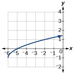
14. \(f(x) = \frac{1}{x + 2} - 1\)

For the following exercises, determine whether the functions are even, odd, or neither.

15. \(f(x) = - \frac{5}{x^{2}} + 9x^{6}\)

Solution (click to reveal)

\(\text{even}\)

16. \(f(x) = - \frac{5}{x^{3}} + 9x^{5}\)

17. \(f(x) = \frac{1}{x}\)

Solution (click to reveal)

\(\text{odd}\)

18. Graph the absolute value function \(f(x) = - 2\left| {x - 1} \right| + 3.\)

For the following exercises, find the inverse of the function.

19. \(f(x) = 3x - 5\)

Solution (click to reveal)

\(f^{- 1}(x) = \frac{x + 5}{3}\)

20. \(f(x) = \frac{4}{x + 7}\)

For the following exercises, use the graph of \(g\) shown in .

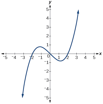
21. On what intervals is the function increasing?

Solution (click to reveal)

\(( - \infty, - 1.1)\mspace{9mu}\text{and~}(1.1,\infty)\)

22. On what intervals is the function decreasing?

23. Approximate the local minimum of the function. Express the answer as an ordered pair. The ordered pair should include both the \(x\) value as well as the \(g(x)\) value.

Solution (click to reveal)

\(\left( {1.1, - 0.9} \right)\)

24. Approximate the local maximum of the function. Express the answer as an ordered pair. The ordered pair should include both the \(x\) value as well as the \(g(x)\) value.

For the following exercises, use the graph of the piecewise function shown in .

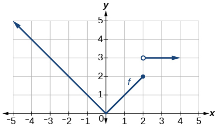
25. Find \(f(2).\)

Solution (click to reveal)

\(f(2) = 2\)

26. Find \(f(-2).\)

27. Write an equation for the piecewise function.

Solution (click to reveal)

\(f(x) = \left\{ \begin{matrix} {|x|\mspace{9mu}\mspace{9mu}\mspace{9mu}\text{if}\mspace{9mu}\mspace{9mu} x \leq 2} \\ {3\mspace{9mu}\mspace{9mu}\mspace{9mu}\mspace{9mu}\mspace{9mu}\text{if}\mspace{9mu}\mspace{9mu} x > 2} \end{matrix} \right.\)

For the following exercises, use the values listed in .

\(x\)	0	1	2	3	4	5	6	7	8
\(F(x)\)	1	3	5	7	9	11	13	15	17

28. Find \(f(6).\)

29. Solve the equation \(f(x) = 5.\)

Solution (click to reveal)

\(x = 2\)

30. Is the graph increasing or decreasing on its domain?

31. Is the function represented by the graph one-to-one?

Solution (click to reveal)

yes

32. Find \(f^{- 1}(15).\)

33. Given \(f(x) = - 2x + 11,\) find \(f^{- 1}(x).\)

Solution (click to reveal)

\(f^{- 1}(x) = - \frac{x - 11}{2}\)