A | Proofs, Identities, and Toolkit Functions
Important Proofs and Derivations
Product Rule
\(\log_{a}xy = \log_{a}x + \log_{a}y\)
where \(x\) and \(y\) are positive, and \(a > 0,a \neq 1.\)
Proof:
Let \(m = \log_{a}x\) and \(n = \log_{a}y.\)
Write in exponent form.
\(x = a^{m}\) and \(y = a^{n}.\)
Multiply.
\(xy = a^{m}a^{n} = a^{m + n}\)
\(\begin{array}{ccl} a^{m + n} & = & {xy} \\ {\log_{a}(xy)} & = & {m + n} \\ & = & {\log_{a}x + \log_{a}y} \end{array}\)
Change of Base Rule
\(\begin{array}{l} \\ {\log_{a}b = \frac{\log_{c}b}{\log_{c}a}} \\ {\log_{a}b = \frac{1}{\log_{b}a}} \end{array}\)
where \(a, b, c\) are positive, and \(a \neq 1, b \neq 1, c \neq 1.\)
Proof:
Let \(x = \log_{a}b.\)
Write in exponent form.
\(a^{x} = b\)
Take the \(\log_{c}\) of both sides.
\(\begin{array}{rcl} {\log_{c}a^{x}} & = & {\log_{c}b} \\ {x\log_{c}a} & = & {\log_{c}b} \\ x & = & \frac{\log_{c}b}{\log_{c}a} \\ {\log_{a}b} & = & \frac{\log_{c}b}{\log_{c}a} \end{array}\)
When \(c = b,\)
\(\log_{a}b = \frac{\log_{b}b}{\log_{b}a} = \frac{1}{\log_{b}a}\)
Heron’s Formula
\(A = \sqrt{s\left( {s - a} \right)\left( {s - b} \right)\left( {s - c} \right)}\)
where \(s = \frac{a + b + c}{2}\)
Proof:
Let \(a,\) \(b,\) and \(c\) be the sides of a triangle, and \(h\) be the height.
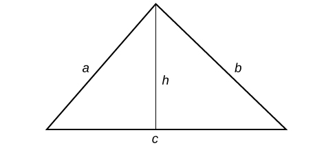
So \(s = \frac{a + b + c}{2}\).
We can further name the parts of the base in each triangle established by the height such that \(p + q = c.\)
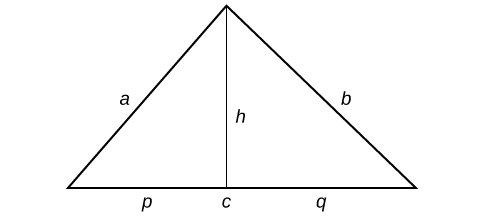
Using the Pythagorean Theorem, \(h^{2} + p^{2} = a^{2}\) and \(h^{2} + q^{2} = b^{2}.\)
Since \(q = c - p,\) then \(q^{2} = \left( {c - p} \right)^{2}.\) Expanding, we find that \(q^{2} = c^{2} - 2cp + p^{2}.\)
We can then add \(h^{2}\) to each side of the equation to get \(h^{2} + q^{2} = h^{2} + c^{2} - 2cp + p^{2}.\)
Substitute this result into the equation \(h^{2} + q^{2} = b^{2}\) yields \(b^{2} = h^{2} + c^{2} - 2cp + p^{2}.\)
Then replacing \(h^{2} + p^{2}\) with \(a^{2}\) gives \(b^{2} = a^{2} - 2cp + c^{2}.\)
Solve for \(p\) to get
\(p = \frac{a^{2} - b^{2} - c^{2}}{2c}\)
Since \(h^{2} = a^{2} - p^{2},\) we get an expression in terms of \(a,\) \(b,\) and \(c.\)
\(\begin{array}{ccl} h^{2} & = & {a^{2} - p^{2}} \\ & = & {(a + p)(a - p)} \\ & = & {\left\lbrack {a + \frac{\left( {a^{2} + c^{2} - b^{2}} \right)}{2c}} \right\rbrack\left\lbrack {a - \frac{\left( {a^{2} + c^{2} - b^{2}} \right)}{2c}} \right\rbrack} \\ & = & \frac{\left( {2ac + a^{2} + c^{2} - b^{2}} \right)\left( {2ac - a^{2} - c^{2} + b^{2}} \right)}{4c^{2}} \\ & = & \frac{\left( {{(a + c)}^{2} - b^{2}} \right)\left( {b^{2} - {(a - c)}^{2}} \right)}{4c^{2}} \\ & = & \frac{(a + b + c)(a + c - b)(b + a - c)(b - a + c)}{4c^{2}} \\ & = & \frac{(a + b + c)( - a + b + c)(a - b + c)(a + b - c)}{4c^{2}} \\ & = & \frac{2s \cdot (2s - a) \cdot (2s - b)(2s - c)}{4c^{2}} \end{array}\)
Therefore,
\(\begin{array}{rcl} h^{2} & = & \frac{4s(s - a)(s - b)(s - c)}{c^{2}} \\ h & = & \frac{2\sqrt{s(s - a)(s - b)(s - c)}}{c} \end{array}\)
And since \(A = \frac{1}{2}ch,\) then
\(\begin{array}{ccl} A & = & {\frac{1}{2}c\frac{2\sqrt{s(s - a)(s - b)(s - c)}}{c}} \\ & = & \sqrt{s(s - a)(s - b)(s - c)} \end{array}\)
Properties of the Dot Product
\(\mathbf{u} \cdot \mathbf{v} = \mathbf{v} \cdot \mathbf{u}\)
- Proof:
\(\begin{array}{cl} {\mathbf{u} \cdot \mathbf{v}} & {= \left\langle \mathbf{u}_{1},\mathbf{u}_{2},...\mathbf{u}_{n} \right\rangle \cdot \left\langle \mathbf{v}_{1},\mathbf{v}_{2},...\mathbf{v}_{n} \right\rangle} \\ & {= \mathbf{u}_{1}\mathbf{v}_{1} + \mathbf{u}_{2}\mathbf{v}_{2} + ... + \mathbf{u}_{n}\mathbf{v}_{n}} \\ & {= \mathbf{v}_{1}\mathbf{u}_{1} + \mathbf{v}_{2}\mathbf{u}_{2} + ... + \mathbf{v}_{n}\mathbf{u}_{n}} \\ & {= \left\langle \mathbf{v}_{1},\mathbf{v}_{2},...\mathbf{v}_{n} \right\rangle \cdot \left\langle \mathbf{u}_{1},\mathbf{u}_{2},...\mathbf{u}_{n} \right\rangle} \\ & {= \mathbf{v} \cdot \mathbf{u}} \end{array}\)
\(\mathbf{u} \cdot \left( {\mathbf{v} + w} \right) = \mathbf{u} \cdot \mathbf{v} + \mathbf{u} \cdot w\)
- Proof:
\(\begin{array}{cl} {\mathbf{u} \cdot (\mathbf{v} + \mathbf{w})} & {= \left\langle \mathbf{u}_{1},\mathbf{u}_{2},...\mathbf{u}_{n} \right\rangle \cdot \left( {\left\langle \mathbf{v}_{1},\mathbf{v}_{2},...\mathbf{v}_{n} \right\rangle + \left\langle \mathbf{w}_{1},\mathbf{w}_{2},...\mathbf{w}_{n} \right\rangle} \right)} \\ & {= \left\langle \mathbf{u}_{1},\mathbf{u}_{2},...\mathbf{u}_{n} \right\rangle \cdot \left\langle \mathbf{v}_{1} + \mathbf{w}_{1},\mathbf{v}_{2} + \mathbf{w}_{2},...\mathbf{v}_{n} + \mathbf{w}_{n} \right\rangle} \\ & = \mathbf{u}_{1}(\mathbf{v}_{1} + \mathbf{w}_{1})+\mathbf{u}_{2}(\mathbf{v}_{2} + \mathbf{w}_{2})+...+\mathbf{u}_{n}(\mathbf{v}_{n} + \mathbf{w}_{n}) \\ & {= \mathbf{u}_{1}\mathbf{v}_{1} + \mathbf{u}_{1}\mathbf{w}_{1}+\mathbf{u}_{2}\mathbf{v}_{2} + \mathbf{u}_{2}\mathbf{w}_{2}+...+\mathbf{u}_{n}\mathbf{v}_{n} + \mathbf{u}_{n}\mathbf{w}_{n} } \\ & {= ( \mathbf{u}_{1}\mathbf{v}_{1}+\mathbf{u}_{2}\mathbf{v}_{2}+...+\mathbf{u}_{n}\mathbf{v}_{n} ) + (\mathbf{u}_{1}\mathbf{w}_{1}+\mathbf{u}_{2}\mathbf{w}_{2}+...+\mathbf{u}_{n}\mathbf{w}_{n} )} \\ & {= \left\langle \mathbf{u}_{1},\mathbf{u}_{2},...\mathbf{u}_{n} \right\rangle \cdot \left\langle \mathbf{v}_{1},\mathbf{v}_{2},...\mathbf{v}_{n} \right\rangle + \left\langle \mathbf{u}_{1},\mathbf{u}_{2},...\mathbf{u}_{n} \right\rangle \cdot \left\langle \mathbf{w}_{1},\mathbf{w}_{2},...\mathbf{w}_{n} \right\rangle} \\ & {= \mathbf{u} \cdot \mathbf{v} + \mathbf{u} \cdot \mathbf{w}} \end{array}\)
\(\mathbf{u} \cdot \mathbf{u} = \left| \mathbf{u} \right|^{2}\)
- Proof:
\(\begin{array}{cl} {\mathbf{u} \cdot \mathbf{u}} & {= \left\langle \mathbf{u}_{1},\mathbf{u}_{2},...\mathbf{u}_{n} \right\rangle \cdot \left\langle \mathbf{u}_{1},\mathbf{u}_{2},...\mathbf{u}_{n} \right\rangle} \\ & {= \mathbf{u}_{1}\mathbf{u}_{1} + \mathbf{u}_{2}\mathbf{u}_{2} + ... + \mathbf{u}_{n}\mathbf{u}_{n}} \\ & {= \mathbf{u}_{1}{}^{2} + \mathbf{u}_{2}{}^{2} + ... + \mathbf{u}_{n}{}^{2}} \\ & \left. = \middle| \left\langle \mathbf{u}_{1},\mathbf{u}_{2},...\mathbf{u}_{n} \right\rangle|^{2} \right. \\ & {= \mathbf{u} \cdot \mathbf{u}} \end{array}\)
Standard Form of the Ellipse centered at the Origin
\(1 = \frac{x^{2}}{a^{2}} + \frac{y^{2}}{b^{2}}\)
Derivation
An ellipse consists of all the points for which the sum of distances from two foci is constant:
\(\sqrt{\left( {x - \left( {- c} \right)} \right)^{2} + \left( {y - 0} \right)^{2}} + \sqrt{\left( {x - c} \right)^{2} + \left( {y - 0} \right)^{2}} = \text{constant}\)
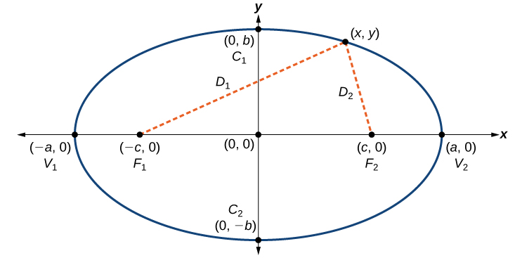
Consider a vertex.
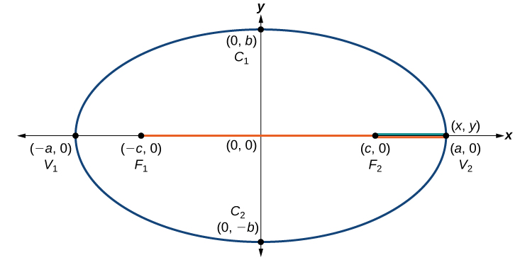
Then, \(\sqrt{\left( {x - \left( {- c} \right)} \right)^{2} + \left( {y - 0} \right)^{2}} + \sqrt{\left( {x - c} \right)^{2} + \left( {y - 0} \right)^{2}} = 2a\)
Consider a covertex.
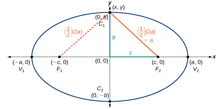
Then \(b^{2} + c^{2} = a^{2}.\)
\(\begin{array}{rcl} {\sqrt{{(x - ( - c))}^{2} + {(y - 0)}^{2}} + \sqrt{{(x - c)}^{2} + {(y - 0)}^{2}}} & = & {2a} \\ \sqrt{{(x + c)}^{2} + y^{2}} & = & {2a - \sqrt{{(x - c)}^{2} + y^{2}}} \\ {{(x + c)}^{2} + y^{2}} & = & \left( {2a - \sqrt{{(x - c)}^{2} + y^{2}}} \right)^{2} \\ {x^{2} + 2cx + c^{2} + y^{2}} & = & {4a^{2} - 4a\sqrt{{(x - c)}^{2} + y^{2}} + {(x - c)}^{2} + y^{2}} \\ {x^{2} + 2cx + c^{2} + y^{2}} & = & {4a^{2} - 4a\sqrt{{(x - c)}^{2} + y^{2}} + x^{2} - 2cx + y^{2}} \\ {2cx} & = & {4a^{2} - 4a\sqrt{{(x - c)}^{2} + y^{2}} - 2cx} \\ {4cx - 4a^{2}} & = & {4a\sqrt{{(x - c)}^{2} + y^{2}}} \\ {- \frac{1}{4a}\left( {4cx - 4a^{2}} \right)} & = & \sqrt{{(x - c)}^{2} + y^{2}} \\ {a - \frac{c}{a}x} & = & \sqrt{{(x - c)}^{2} + y^{2}} \\ {a^{2} - 2xc + \frac{c^{2}}{a^{2}}x^{2}} & = & {{(x - c)}^{2} + y^{2}} \\ {a^{2} - 2xc + \frac{c^{2}}{a^{2}}x^{2}} & = & {x^{2} - 2xc + c^{2} + y^{2}} \\ {a^{2} + \frac{c^{2}}{a^{2}}x^{2}} & = & {x^{2} + c^{2} + y^{2}} \\ {a^{2} + \frac{c^{2}}{a^{2}}x^{2}} & = & {x^{2} + c^{2} + y^{2}} \\ {a^{2} - c^{2}} & = & {x^{2} - \frac{c^{2}}{a^{2}}x^{2} + y^{2}} \\ {a^{2} - c^{2}} & = & {x^{2}\left( {1 - \frac{c^{2}}{a^{2}}} \right) + y^{2}} \end{array}\)
Let \(1 = \frac{a^{2}}{a^{2}}.\)
\[\begin{array}{rcl} {a^{2} - c^{2}} & = & {x^{2}\left( \frac{a^{2} - c^{2}}{a^{2}} \right) + y^{2}} \\ 1 & = & {\frac{x^{2}}{a^{2}} + \frac{y^{2}}{a^{2} - c^{2}}} \end{array}\]
Because \(b^{2} + c^{2} = a^{2},\) then \(b^{2} = a^{2} - c^{2}.\)
\[\begin{array}{rcl} 1 & = & {\frac{x^{2}}{a^{2}} + \frac{y^{2}}{a^{2} - c^{2}}} \\ 1 & = & {\frac{x^{2}}{a^{2}} + \frac{y^{2}}{b^{2}}} \end{array}\]
Standard Form of the Hyperbola
\(1 = \frac{x^{2}}{a^{2}} - \frac{y^{2}}{b^{2}}\)
Derivation
A hyperbola is the set of all points in a plane such that the absolute value of the difference of the distances between two fixed points is constant.
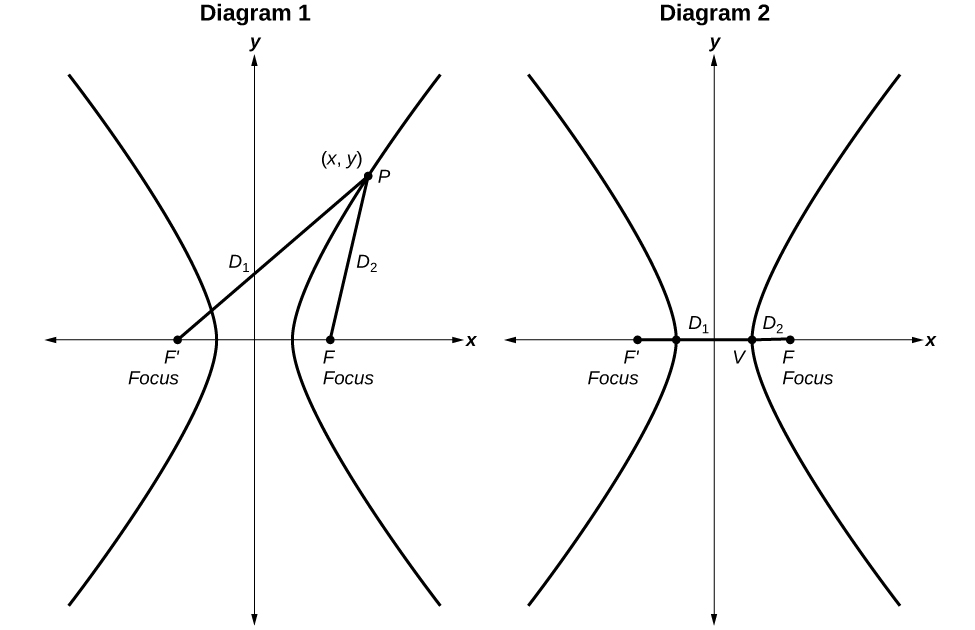
Diagram 1: The difference of the distances from Point \(P\) to the foci is constant:
\(\sqrt{{(x - ( - c))}^{2} + {(y - 0)}^{2}} - \sqrt{{(x - c)}^{2} + {(y - 0)}^{2}} = \text{constant}\)
Diagram 2: When the point is a vertex, the difference is \(2a.\)
\(\sqrt{\left( {x - \left( {- c} \right)} \right)^{2} + \left( {y - 0} \right)^{2}} - \sqrt{\left( {x - c} \right)^{2} + \left( {y - 0} \right)^{2}} = 2a\)
\(\begin{array}{rcl} {\sqrt{{(x - ( - c))}^{2} + {(y - 0)}^{2}} - \sqrt{{(x - c)}^{2} + {(y - 0)}^{2}}} & = & {2a} \\ {\sqrt{{(x + c)}^{2} + y^{2}} - \sqrt{{(x - c)}^{2} + y^{2}}} & = & {2a} \\ \sqrt{{(x + c)}^{2} + y^{2}} & = & {2a + \sqrt{{(x - c)}^{2} + y^{2}}} \\ {{(x + c)}^{2} + y^{2}} & = & \left( {2a + \sqrt{{(x - c)}^{2} + y^{2}}} \right) \\ {x^{2} + 2cx + c^{2} + y^{2}} & = & {4a^{2} + 4a\sqrt{{(x - c)}^{2}} + y^{2}} \\ {x^{2} + 2cx + c^{2} + y^{2}} & = & {4a^{2} + 4a\sqrt{{(x - c)}^{2} + y^{2}} + x^{2} - 2cx + y^{2}} \\ {2cx} & = & {4a^{2} + 4a\sqrt{{(x - c)}^{2} + y^{2}} - 2cx} \\ {4cx - 4a^{2}} & = & {4a\sqrt{{(x - c)}^{2} + y^{2}}} \\ {cx - a^{2}} & = & {a\sqrt{{(x - c)}^{2} + y^{2}}} \\ \left( {cx - a^{2}} \right)^{2} & = & {a^{2}\left( {{(x - c)}^{2} + y^{2}} \right)} \\ {c^{2}x^{2} - 2a^{2}c^{2}x^{2} + a^{4}} & = & {a^{2}x^{2} - 2a^{2}c^{2}x^{2} + a^{2}c^{2} + a^{2}y^{2}} \\ {c^{2}x^{2} + a^{4}} & = & {a^{2}x^{2} + a^{2}c^{2} + a^{2}y^{2}} \\ {a^{4} - a^{2}c^{2}} & = & {a^{2}x^{2} - c^{2}x^{2} + a^{2}y^{2}} \\ {a^{2}\left( {a^{2} - c^{2}} \right)} & = & {\left( {a^{2} - c^{2}} \right)x^{2} + a^{2}y^{2}} \\ {a^{2}\left( {a^{2} - c^{2}} \right)} & = & {\left( {c^{2} - a^{2}} \right)x^{2} - a^{2}y^{2}} \end{array}\)
Define \(b\) as a positive number such that \(b^{2} = c^{2} - a^{2}.\)
\[\begin{array}{rcl} {a^{2}b^{2}} & = & {b^{2}x^{2} - a^{2}y^{2}} \\ \frac{a^{2}b^{2}}{a^{2}b^{2}} & = & {\frac{b^{2}x^{2}}{a^{2}b^{2}} - \frac{a^{2}y^{2}}{a^{2}b^{2}}} \\ 1 & = & {\frac{x^{2}}{a^{2}} - \frac{y^{2}}{b^{2}}} \end{array}\]
Trigonometric Identities
| Pythagorean Identities | \(\begin{array}{l} {\cos^{2}\theta + \sin^{2}\theta = 1} \\ {1 + \tan^{2}\theta = \sec^{2}\theta} \\ {1 + \cot^{2}\theta = \csc^{2}\theta} \end{array}\) |
| Even-Odd Identities | \(\begin{array}{l} {\cos\operatorname{(-}\theta) = \cos\;\theta} \\ {\sec\operatorname{(-}\theta) = \sec\;\theta} \\ {\sin\operatorname{(-}\theta) = - \sin\;\theta} \\ {\tan\operatorname{(-}\theta) = - \tan\;\theta} \\ {\csc\operatorname{(-}\theta) = - \csc\;\theta} \\ {\cot\operatorname{(-}\theta) = - \cot\;\theta} \end{array}\) |
| Cofunction Identities | \(\begin{array}{l} {\cos\;\theta = \sin\left( {\frac{\pi}{2} - \theta} \right)} \\ {\sin\;\theta = \cos\left( {\frac{\pi}{2} - \theta} \right)} \\ {\tan\;\theta = \cot\left( {\frac{\pi}{2} - \theta} \right)} \\ {\cot\;\theta = \tan\left( {\frac{\pi}{2} - \theta} \right)} \\ {\sec\;\theta = \csc\left( {\frac{\pi}{2} - \theta} \right)} \\ {\csc\;\theta = \sec\left( {\frac{\pi}{2} - \theta} \right)} \end{array}\) |
| Fundamental Identities | \(\begin{array}{l} {\tan\;\theta = \frac{\sin\;\theta}{\cos\;\theta}} \\ {\sec\;\theta = \frac{1}{\cos\;\theta}} \\ {\csc\;\theta = \frac{1}{\sin\;\theta}} \\ {\text{cot}\;\theta = \frac{1}{\text{tan}\;\theta} = \frac{\text{cos}\;\theta}{\text{sin}\;\theta}} \end{array}\) |
| Sum and Difference Identities | \(\begin{array}{l} {\cos(\alpha + \beta) = \cos\;\alpha\;\cos\;\beta - \sin\;\alpha\;\sin\;\beta} \\ {\cos(\alpha - \beta) = \cos\;\alpha\;\cos\;\beta + \sin\;\alpha\;\sin\;\beta} \\ {\sin(\alpha + \beta) = \sin\;\alpha\;\cos\;\beta + \cos\;\alpha\;\sin\;\beta} \\ {\sin(\alpha - \beta) = \sin\;\alpha\;\cos\;\beta - \cos\;\alpha\;\sin\;\beta} \\ {\tan(\alpha + \beta) = \frac{\tan\;\alpha + \tan\;\beta}{1 - \tan\;\alpha\;\tan\;\beta}} \\ {\tan(\alpha - \beta) = \frac{\tan\;\alpha - \tan\;\beta}{1 + \tan\;\alpha\;\tan\;\beta}} \end{array}\) |
| Double-Angle Formulas | \(\begin{array}{l} {\sin(2\theta) = 2\;\sin\;\theta\;\cos\;\theta} \\ {\cos(2\theta) = \cos^{2}\theta - \sin^{2}\theta} \\ {\cos(2\theta) = 1 - 2\;\sin^{2}\theta} \\ {\cos(2\theta) = 2\;\cos^{2}\theta - 1} \\ {\tan(2\theta) = \frac{2\;\tan\;\theta}{1 - \tan^{2}\theta}} \end{array}\) |
| Half-Angle Formulas | \(\begin{array}{l} {\sin\;\frac{\alpha}{2} = \pm \sqrt{\frac{1 - \cos\;\alpha}{2}}} \\ {\cos\;\frac{\alpha}{2} = \pm \sqrt{\frac{1 + \cos\;\alpha}{2}}} \\ {\tan\;\frac{\alpha}{2} = \pm \sqrt{\frac{1 - \cos\;\alpha}{1 + \cos\;\alpha}}} \\ {\tan\;\frac{\alpha}{2} = \frac{\sin\;\alpha}{1 + \cos\;\alpha}} \\ {\tan\;\frac{\alpha}{2} = \frac{1 - \cos\;\alpha}{\sin\;\alpha}} \end{array}\) |
| Reduction Formulas | \(\begin{array}{l} {\sin^{2}\theta = \frac{1 - \cos\left( {2\theta} \right)}{2}} \\ {\cos^{2}\theta = \frac{1 + \cos\left( {2\theta} \right)}{2}} \\ {\tan^{2}\theta = \frac{1 - \cos\left( {2\theta} \right)}{1 + \cos\left( {2\theta} \right)}} \end{array}\) |
| Product-to-Sum Formulas | \(\begin{array}{l} {\cos\;\alpha\;\cos\;\beta = \frac{1}{2}\left\lbrack {\cos(\alpha - \beta) + \cos(\alpha + \beta)} \right\rbrack} \\ {\sin\;\alpha\;\cos\;\beta = \frac{1}{2}\left\lbrack {\sin(\alpha + \beta) + \sin(\alpha - \beta)} \right\rbrack} \\ {\sin\;\alpha\;\sin\;\beta = \frac{1}{2}\left\lbrack {\cos(\alpha - \beta) - \cos(\alpha + \beta)} \right\rbrack} \\ {\cos\;\alpha\;\sin\;\beta = \frac{1}{2}\left\lbrack {\sin(\alpha + \beta) - \sin(\alpha - \beta)} \right\rbrack} \end{array}\) |
| Sum-to-Product Formulas | \(\begin{array}{l} {\sin\;\alpha + \sin\;\beta = 2\;\sin\left( \frac{\alpha + \beta}{2} \right)\;\cos\left( \frac{\alpha - \beta}{2} \right)} \\ {\sin\;\alpha - \sin\;\beta = 2\;\sin\left( \frac{\alpha - \beta}{2} \right)\;\cos\left( \frac{\alpha + \beta}{2} \right)} \\ {\cos\;\alpha - \cos\;\beta = - 2\;\sin\left( \frac{\alpha + \beta}{2} \right)\;\sin\left( \frac{\alpha - \beta}{2} \right)} \\ {\cos\;\alpha + \cos\;\beta = 2\;\cos\left( \frac{\alpha + \beta}{2} \right)\;\cos\left( \frac{\alpha - \beta}{2} \right)} \end{array}\) |
| Law of Sines | \(\begin{array}{l} {\frac{\sin\;\alpha}{a} = \frac{\sin\;\beta}{b} = \frac{\sin\;\gamma}{c}} \\ {\frac{a}{\sin\;\alpha} = \frac{b}{\sin\;\beta} = \frac{c}{\sin\;\gamma}} \end{array}\) |
| Law of Cosines | \(\begin{array}{l} {a^{2} = b^{2} + c^{2} - 2bc\;\cos\;\alpha} \\ {b^{2} = a^{2} + c^{2} - 2ac\;\cos\;\beta} \\ {c^{2} = a^{2} + b^{2} - 2ab\;\text{cos}\;\gamma} \end{array}\) |
Table A1
ToolKit Functions
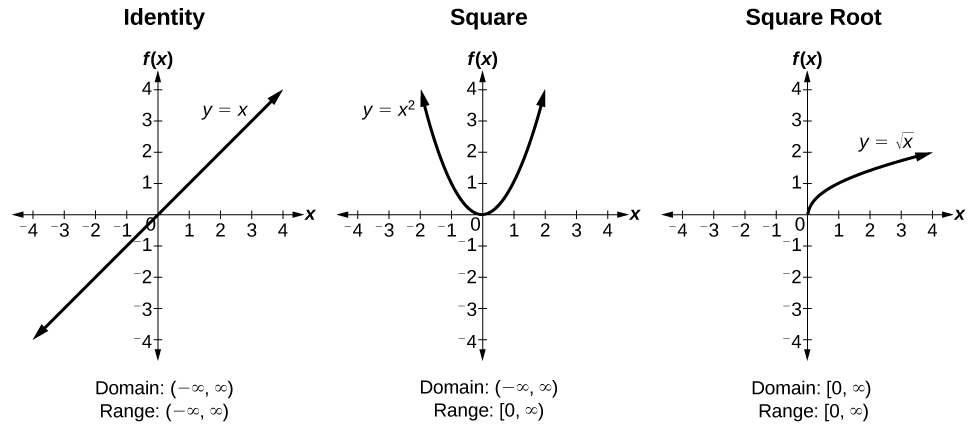
Figure A1
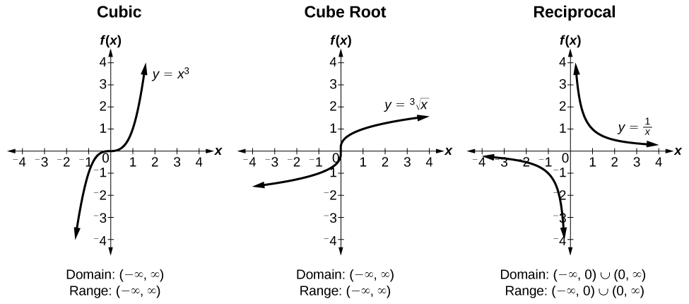
Figure A2
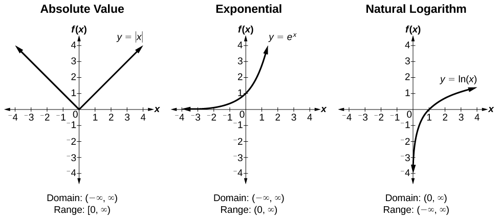
Figure A3
Trigonometric Functions
Unit Circle
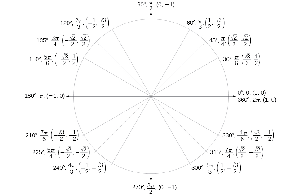
Figure A4
| Angle | \(0\) | \(\frac{\pi}{6},\text{or~30}{^\circ}\) | \(\frac{\pi}{4},\text{or~45}{^\circ}\) | \(\frac{\pi}{3},\text{or~60}{^\circ}\) | \(\frac{\pi}{2},\text{or~90}{^\circ}\) |
|---|---|---|---|---|---|
| Cosine | 1 | \(\frac{\sqrt{3}}{2}\) | \(\frac{\sqrt{2}}{2}\) | \(\frac{1}{2}\) | 0 |
| Sine | 0 | \(\frac{1}{2}\) | \(\frac{\sqrt{2}}{2}\) | \(\frac{\sqrt{3}}{2}\) | 1 |
| Tangent | 0 | \(\frac{\sqrt{3}}{3}\) | 1 | \(\sqrt{3}\) | Undefined |
| Secant | 1 | \(\frac{2\sqrt{3}}{3}\) | \(\sqrt{2}\) | 2 | Undefined |
| Cosecant | Undefined | 2 | \(\sqrt{2}\) | \(\frac{2\sqrt{3}}{3}\) | 1 |
| Cotangent | Undefined | \(\sqrt{3}\) | 1 | \(\frac{\sqrt{3}}{3}\) | 0 |
Table A2