4.1 Angles
A golfer swings to hit a ball over a sand trap and onto the green. An airline pilot maneuvers a plane toward a narrow runway. A dress designer creates the latest fashion. What do they all have in common? They all work with angles, and so do all of us at one time or another. Sometimes we need to measure angles exactly with instruments. Other times we estimate them or judge them by eye. Either way, the proper angle can make the difference between success and failure in many undertakings. In this section, we will examine properties of angles.
4.1.1 Drawing Angles in Standard Position
Properly defining an angle first requires that we define a ray. A ray is a directed line segment. It consists of one point on a line and all points extending in one direction from that point. The first point is called the endpoint of the ray. We can refer to a specific ray by stating its endpoint and any other point on it. The ray in Figure 4.1.1 can be named as ray EF, or in symbol form \(\overset{\longrightarrow}{EF}.\)
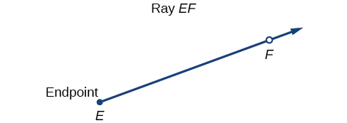
Figure 4.1.1:
An angle is the union of two rays having a common endpoint. The endpoint is called the vertex of the angle, and the two rays are the sides of the angle. The angle in Figure 4.1.2 is formed from \(\overset{\longrightarrow}{ED}\) and \(\overset{\longrightarrow}{EF}\). Angles can be named using a point on each ray and the vertex, such as angle DEF, or in symbol form \(\angle DEF.\)
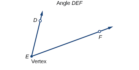
Figure 4.1.2:
Greek letters are often used as variables for the measure of an angle. Table 4.1.3 is a list of Greek letters commonly used to represent angles, and a sample angle is shown in Figure 4.1.4.
| \(\theta\) | \(\varphi\) or \(\phi\) | \(\alpha\) | \(\beta\) | \(\gamma\) |
|---|---|---|---|---|
| theta | phi | alpha | beta | gamma |
Table 4.1.3:
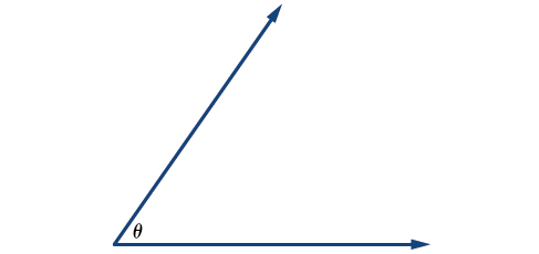
Figure 4.1.4: Angle theta, shown as \(\angle\theta\)
Angle creation is a dynamic process. We start with two rays lying on top of one another. We leave one fixed in place, and rotate the other. The fixed ray is the initial side, and the rotated ray is the terminal side. In order to identify the different sides, we indicate the rotation with a small arrow close to the vertex as in Figure 4.1.5.
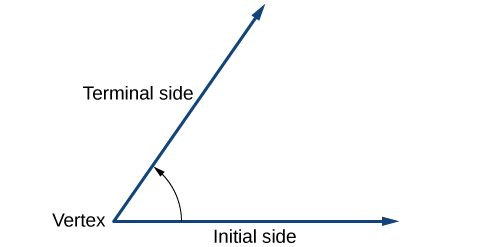
Figure 4.1.5:
As we discussed at the beginning of the section, there are many applications for angles, but in order to use them correctly, we must be able to measure them. The measure of an angle is the amount of rotation from the initial side to the terminal side. Probably the most familiar unit of angle measurement is the degree. One degree is \(\frac{1}{360}\) of a circular rotation, so a complete circular rotation contains \(360\) degrees. An angle measured in degrees should always include the unit “degrees” after the number, or include the degree symbol \({^\circ}.\) For example, \(90\mspace{9mu}\text{degrees} = 90{^\circ}.\)
To formalize our work, we will begin by drawing angles on an \(x\)-\(y\) coordinate plane. Angles can occur in any position on the coordinate plane, but for the purpose of comparison, the convention is to illustrate them in the same position whenever possible. An angle is in standard position if its vertex is located at the origin, and its initial side extends along the positive \(x\)-axis. See Figure 4.1.6.
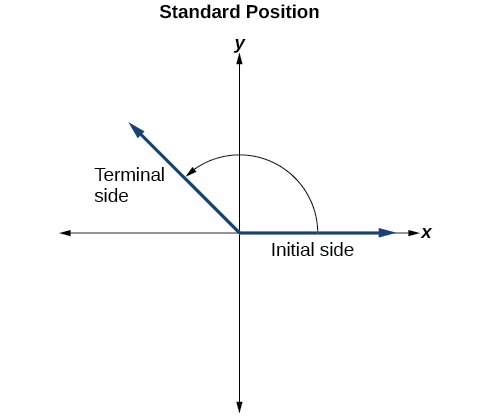
Figure 4.1.6:
If the angle is measured in a counterclockwise direction from the initial side to the terminal side, the angle is said to be a positive angle. If the angle is measured in a clockwise direction, the angle is said to be a negative angle.
Drawing an angle in standard position always starts the same way—draw the initial side along the positive \(x\)-axis. To place the terminal side of the angle, we must calculate the fraction of a full rotation the angle represents. We do that by dividing the angle measure in degrees by \(360{^\circ}.\) For example, to draw a \(90{^\circ}\) angle, we calculate that \(\frac{90{^\circ}\operatorname{}}{360{^\circ}} = \frac{1}{4}.\) So, the terminal side will be one-fourth of the way around the circle, moving counterclockwise from the positive \(x\)-axis. To draw a \(360{^\circ}\operatorname{}\) angle, we calculate that \(\frac{360{^\circ}}{360{^\circ}} = 1.\) So the terminal side will be 1 complete rotation around the circle, moving counterclockwise from the positive \(x\)-axis. In this case, the initial side and the terminal side overlap. See Figure 4.1.7.
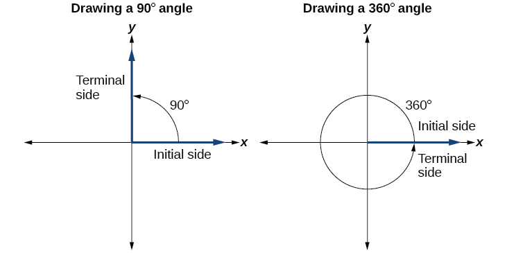
Figure 4.1.7:
Since we define an angle in standard position by its terminal side, we have a special type of angle whose terminal side lies on an axis, a quadrantal angle. This type of angle can have a measure of 0°, 90°, 180°, 270°, or 360°. See Figure 4.1.8.
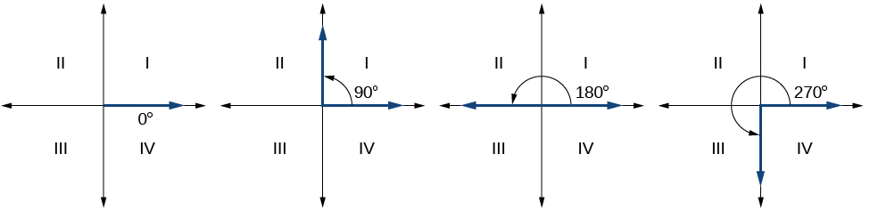
Figure 4.1.8: Quadrantal angles have a terminal side that lies along an axis. Examples are shown.
ⓐ Sketch an angle of \(30{^\circ}\) in standard position.
ⓑ Sketch an angle of \(-135{^\circ}\) in standard position.
Solution (click to reveal)
ⓐ Divide the angle measure by \(360{^\circ}.\)
\[\frac{30{^\circ}}{360{^\circ}} = \frac{1}{12}\]
To rewrite the fraction in a more familiar fraction, we can recognize that
\[\frac{1}{12} = \frac{1}{3}\left( \frac{1}{4} \right)\]
One-twelfth equals one-third of a quarter, so by dividing a quarter rotation into thirds, we can sketch a line at \(30{^\circ},\) as in Figure 8.
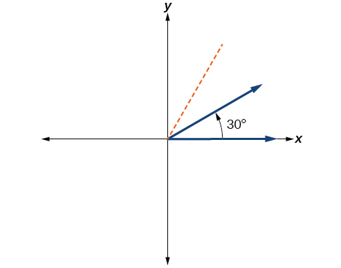
Figure 8
ⓑ Divide the angle measure by \(360{^\circ}.\)
\[\frac{-135{^\circ}}{360{^\circ}} = - \frac{3}{8}\]
In this case, we can recognize that
\[- \frac{3}{8} = - \frac{3}{2}\left( \frac{1}{4} \right)\]
Three-eighths is one and one-half times a quarter, so we place a line by moving clockwise one full quarter and one-half of another quarter, as in Figure 9.
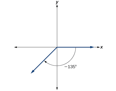
Figure 9
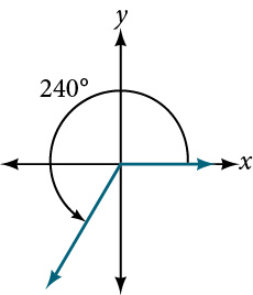
Show an angle of \(240{^\circ}\) on a circle in standard position.
Solution (click to reveal)
4.1.2 Converting Between Degrees and Radians
Dividing a circle into 360 parts is an arbitrary choice, although it creates the familiar degree measurement. We may choose other ways to divide a circle. To find another unit, think of the process of drawing a circle. Imagine that you stop before the circle is completed. The portion that you drew is referred to as an arc. An arc may be a portion of a full circle, a full circle, or more than a full circle, represented by more than one full rotation. The length of the arc around an entire circle is called the circumference of that circle.
The circumference of a circle is \(C = 2\pi r.\) If we divide both sides of this equation by \(r,\) we create the ratio of the circumference, which is always \(2\pi,\) to the radius, regardless of the length of the radius. So the circumference of any circle is \(2\pi \approx 6.28\) times the length of the radius. That means that if we took a string as long as the radius and used it to measure consecutive lengths around the circumference, there would be room for six full string-lengths and a little more than a quarter of a seventh, as shown in Figure 4.1.13.
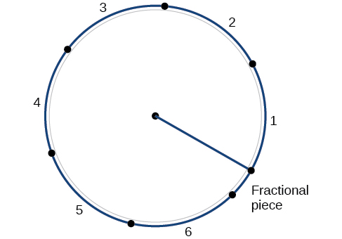
Figure 4.1.13:
This brings us to our new angle measure. One radian is the measure of a central angle of a circle that intercepts an arc equal in length to the radius of that circle. A central angle is an angle formed at the center of a circle by two radii. Because the total circumference equals \(2\pi\) times the radius, a full circular rotation is \(2\pi\) radians.
\[\begin{array}{rcl} {2\pi\mspace{9mu}\text{radians}} & = & 360{^\circ} \\ {\pi\mspace{9mu}\text{radians}} & = & {\frac{360{^\circ}}{2} = 180{^\circ}} \\ {1\mspace{9mu}\text{radian}} & = & {\frac{180{^\circ}}{\pi} \approx 57.3{^\circ}} \end{array}\]
See Figure 4.1.14. Note that when an angle is described without a specific unit, it refers to radian measure. For example, an angle measure of 3 indicates 3 radians. In fact, radian measure is dimensionless, since it is the quotient of a length (circumference) divided by a length (radius) and the length units cancel.
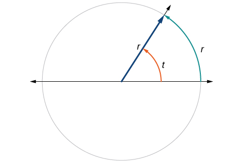
Figure 4.1.14: The angle \(t\) sweeps out a measure of one radian. Note that the length of the intercepted arc is the same as the length of the radius of the circle.
Relating Arc Lengths to Radius
An arc length \(s\) is the length of the curve along the arc. Just as the full circumference of a circle always has a constant ratio to the radius, the arc length produced by any given angle also has a constant relation to the radius, regardless of the length of the radius.
This ratio, called the radian measure, is the same regardless of the radius of the circle—it depends only on the angle. This property allows us to define a measure of any angle as the ratio of the arc length \(s\) to the radius \(r\). See Figure 4.1.15.
\[\begin{matrix} s & = & {r\theta} \\ \theta & = & \frac{s}{r} \end{matrix}\]
If \(s = r,\) then \(\theta = \frac{r}{r} = \mspace{9mu}\text{1~radian}\text{.}\)
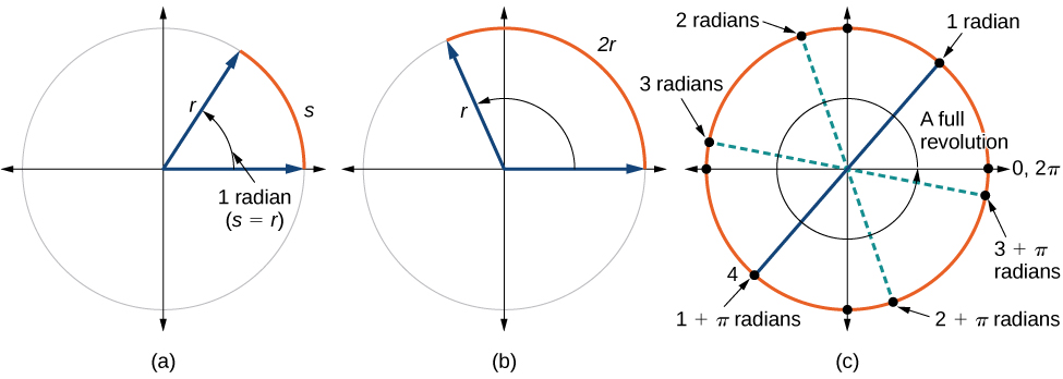
Figure 4.1.15: (a) In an angle of 1 radian, the arc length \(s\) equals the radius \(r.\) (b) An angle of 2 radians has an arc length \(s = 2r.\) (c) A full revolution is \(2\pi,\) or about 6.28 radians.
To elaborate on this idea, consider two circles, one with radius 2 and the other with radius 3. Recall the circumference of a circle is \(C = 2\pi r,\) where \(r\) is the radius. The smaller circle then has circumference \(2\pi(2) = 4\pi\) and the larger has circumference \(2\pi(3) = 6\pi.\) Now we draw a \(45{^\circ}\) angle on the two circles, as in Figure 4.1.16.
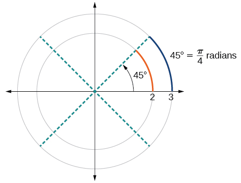
Figure 4.1.16: A \(45{^\circ}\) angle contains one-eighth of the circumference of a circle, regardless of the radius.
Notice what happens if we find the ratio of the arc length divided by the radius of the circle.
\[\begin{matrix} {\text{Smaller~circle:}\mspace{9mu}\frac{\frac{1}{2}\pi}{2}} & = & {\frac{1}{4}\pi} \\ {\text{Larger~circle:}\mspace{9mu}\frac{\frac{3}{4}\pi}{3}} & = & {\frac{1}{4}\pi} \end{matrix}\]
Since both ratios are \(\frac{1}{4}\pi,\) the angle measures of both circles are the same, even though the arc length and radius differ.
Using Radians
Because radian measure is the ratio of two lengths, it is a unitless measure. For example, in Figure 4.1.15, suppose the radius were 2 inches and the distance along the arc were also 2 inches. When we calculate the radian measure of the angle, the “inches” cancel, and we have a result without units. Therefore, it is not necessary to write the label “radians” after a radian measure, and if we see an angle that is not labeled with “degrees” or the degree symbol, we can assume that it is a radian measure.
Considering the most basic case, the unit circle (a circle with radius 1), we know that 1 rotation equals 360 degrees, \(360{^\circ}.\) We can also track one rotation around a circle by finding the circumference, \(C = 2\pi r,\) and for the unit circle \(C = 2\pi.\) These two different ways to rotate around a circle give us a way to convert from degrees to radians.
\[\begin{array}{rclcl} \text{1~rotation} & = & 360{^\circ} & = & {2\pi\mspace{9mu}\text{radians}} \\ {\frac{1}{2}\mspace{9mu}\text{rotation}} & = & 180{^\circ} & = & {\pi\mspace{9mu}\text{radians}} \\ {\frac{1}{4}\mspace{9mu}\text{rotation}} & = & 90{^\circ} & = & {\frac{\pi}{2}\mspace{9mu}\text{radians}} \end{array}\]
Identifying Special Angles Measured in Radians
In addition to knowing the measurements in degrees and radians of a quarter revolution, a half revolution, and a full revolution, there are other frequently encountered angles in one revolution of a circle with which we should be familiar. It is common to encounter multiples of 30, 45, 60, and 90 degrees. These values are shown in Figure 4.1.19. Memorizing these angles will be very useful as we study the properties associated with angles.
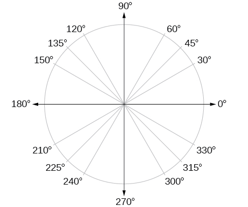
Figure 4.1.19: Commonly encountered angles measured in degrees
Now, we can list the corresponding radian values for the common measures of a circle corresponding to those listed in Figure 4.1.19, which are shown in Figure 4.1.20. Be sure you can verify each of these measures.
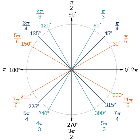
Figure 4.1.20: Commonly encountered angles measured in radians
Converting Between Radians and Degrees
Because degrees and radians both measure angles, we need to be able to convert between them. We can easily do so using a proportion where \(\theta\) is the measure of the angle in degrees and \(\theta_{R}\) is the measure of the angle in radians.
\[\frac{\theta}{180} = \frac{\theta_{{}^{R}}}{\pi}\]
This proportion shows that the measure of angle \(\theta\) in degrees divided by 180 equals the measure of angle \(\theta\) in radians divided by \(\pi.\) Or, phrased another way, degrees is to 180 as radians is to \(\pi.\)
\[\frac{\text{Degrees}}{180} = \frac{\text{Radians}}{\pi}\]
4.1.3 Finding Coterminal Angles
Converting between degrees and radians can make working with angles easier in some applications. For other applications, we may need another type of conversion. Negative angles and angles greater than a full revolution are more awkward to work with than those in the range of \(0{^\circ}\) to \(360{^\circ},\) or \(0\) to \(2\pi.\) It would be convenient to replace those out-of-range angles with a corresponding angle within the range of a single revolution.
It is possible for more than one angle to have the same terminal side. Look at Figure 4.1.28. The angle of \(140{^\circ}\) is a positive angle, measured counterclockwise. The angle of \(–220{^\circ}\) is a negative angle, measured clockwise. But both angles have the same terminal side. If two angles in standard position have the same terminal side, they are coterminal angles. Every angle greater than \(360{^\circ}\) or less than \(0{^\circ}\) is coterminal with an angle between \(0{^\circ}\) and \(360{^\circ},\) and it is often more convenient to find the coterminal angle within the range of \(0{^\circ}\) to \(360{^\circ}\) than to work with an angle that is outside that range.
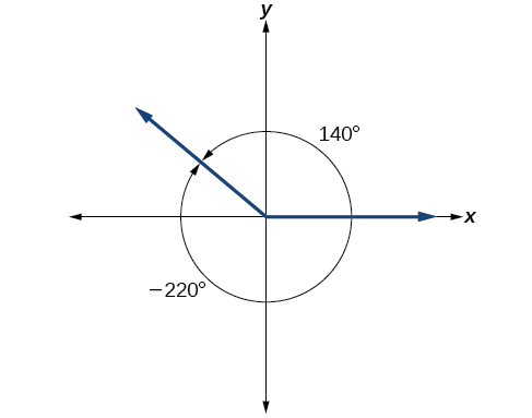
Figure 4.1.28: An angle of \(140{^\circ}\) and an angle of \(–220{^\circ}\) are coterminal angles.
Any angle has infinitely many coterminal angles because each time we add \(360{^\circ}\) to that angle—or subtract \(360{^\circ}\) from it—the resulting value has a terminal side in the same location. For example, \(\text{100°}\) and \(\text{460°}\) are coterminal for this reason, as is \(-260{^\circ}.\)
An angle’s reference angle is the measure of the smallest, positive, acute angle \(t'\) formed by the terminal side of the angle \(t\) and the horizontal axis. Thus positive reference angles have terminal sides that lie in the first quadrant and can be used as models for angles in other quadrants. See Figure 4.1.29 for examples of reference angles for angles in different quadrants.
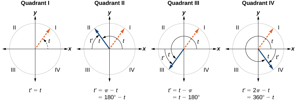
Figure 4.1.29:
Find the least positive angle \(\theta\) that is coterminal with an angle measuring \(800{^\circ},\) where \(0{^\circ} \leq \theta < 360{^\circ}.\)
Solution (click to reveal)
An angle with measure \(800{^\circ}\) is coterminal with an angle with measure \(800 - 360 = 440{^\circ},\) but \(440{^\circ}\operatorname{}\) is still greater than \(360{^\circ},\) so we subtract \(360{^\circ}\) again to find another coterminal angle: \(440 - 360 = 80{^\circ}.\)
The angle \(\theta = 80{^\circ}\) is coterminal with \(800{^\circ}.\) To put it another way, \(800{^\circ}\) equals \(80{^\circ}\) plus two full rotations, as shown in Figure 18.
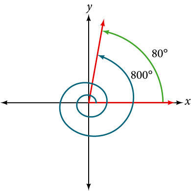
Figure 18
Show the angle with measure \(-45{^\circ}\) on a circle and find a positive coterminal angle \(\alpha\) such that \(0{^\circ} \leq \alpha < 360{^\circ}.\)
Solution (click to reveal)
Since \(45{^\circ}\) is half of \(90{^\circ},\) we can start at the positive horizontal axis and measure clockwise half of a \(90{^\circ}\) angle.
Because we can find coterminal angles by adding or subtracting a full rotation of \(360{^\circ},\) we can find a positive coterminal angle here by adding \(360{^\circ}.\)
\[-45{^\circ} + 360{^\circ} = 315{^\circ}\]
We can then show the angle on a circle, as in Figure 4.1.41.
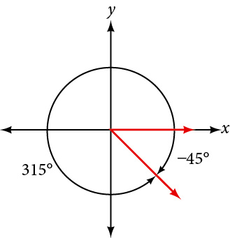
Figure 19
Finding Coterminal Angles Measured in Radians
We can find coterminal angles measured in radians in much the same way as we have found them using degrees. In both cases, we find coterminal angles by adding or subtracting one or more full rotations.
Find an angle \(\beta\) that is coterminal with \(\frac{19\pi}{4},\) where \(0 \leq \beta < 2\pi.\)
Solution (click to reveal)
When working in degrees, we found coterminal angles by adding or subtracting 360 degrees, a full rotation. Likewise, in radians, we can find coterminal angles by adding or subtracting full rotations of \(2\pi\) radians:
\[\begin{array}{ccl} {\frac{19\pi}{4} - 2\pi} & = & {\frac{19\pi}{4} - \frac{8\pi}{4}} \\ & = & \frac{11\pi}{4} \end{array}\]
The angle \(\frac{11\pi}{4}\) is coterminal, but not less than \(2\pi,\) so we subtract another rotation.
\[\begin{array}{ccl} {\frac{11\pi}{4} - 2\pi} & = & {\frac{11\pi}{4} - \frac{8\pi}{4}} \\ & = & \frac{3\pi}{4} \end{array}\]
The angle \(\frac{3\pi}{4}\) is coterminal with \(\frac{19\pi}{4},\) as shown in Figure 4.1.41.
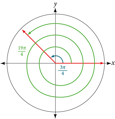
Figure 20
4.1.4 Determining the Length of an Arc
Recall that the radian measure \(\theta\) of an angle was defined as the ratio of the arc length \(s\) of a circular arc to the radius \(r\) of the circle, \(\theta = \frac{s}{r}.\) From this relationship, we can find arc length along a circle, given an angle.
In a circle of radius \(r\), the length of an arc \(s\) subtended by an angle with measure \(\theta\) in radians, shown in Figure 4.1.41, is
\[s = r\theta\]
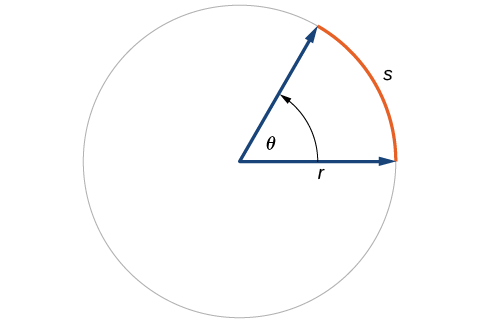
Figure 4.1.41:
4.1.5 Finding the Area of a Sector of a Circle
In addition to arc length, we can also use angles to find the area of a sector of a circle. A sector is a region of a circle bounded by two radii and the intercepted arc, like a slice of pizza or pie. Recall that the area of a circle with radius \(r\) can be found using the formula \(A = \pi r^{2}.\) If the two radii form an angle of \(\theta,\) measured in radians, then \(\frac{\theta}{2\pi}\) is the ratio of the angle measure to the measure of a full rotation and is also, therefore, the ratio of the area of the sector to the area of the circle. Thus, the area of a sector is the fraction \(\frac{\theta}{2\pi}\) multiplied by the entire area. (Always remember that this formula only applies if \(\theta\) is in radians.)
\[\begin{array}{ccl} \text{Area~of~sector} & = & {\left( \frac{\theta}{2\pi} \right)\pi r^{2}} \\ & = & \frac{\theta\pi r^{2}}{2\pi} \\ & = & {\frac{1}{2}\theta r^{2}} \end{array}\]
The area of a sector of a circle with radius \(r\) subtended by an angle \(\theta,\) measured in radians, is
\[A = \frac{1}{2}\theta r^{2}\]
See Figure 4.1.46.
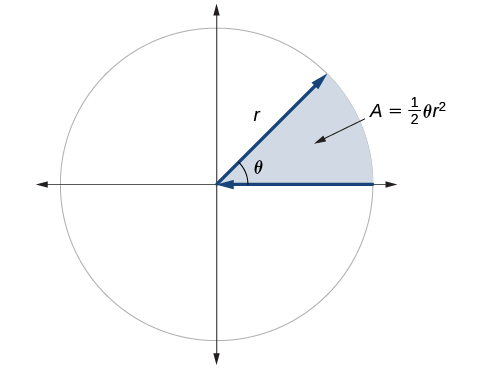
Figure 4.1.46: The area of the sector equals half the square of the radius times the central angle measured in radians.
An automatic lawn sprinkler sprays a distance of 20 feet while rotating 30 degrees, as shown in Figure 4.1.49. What is the area of the sector of grass the sprinkler waters?

Figure 4.1.49: The sprinkler sprays 20 ft within an arc of \(30{^\circ}.\)
Solution (click to reveal)
First, we need to convert the angle measure into radians. Because 30 degrees is one of our special angles, we already know the equivalent radian measure, but we can also convert:
\[\begin{array}{ccl} {30\mspace{9mu}\text{degrees}} & = & {30 \cdot \frac{\pi}{180}} \\ & = & {\frac{\pi}{6}\mspace{9mu}\text{radians}} \end{array}\]
The area of the sector is then
\[\begin{array}{ccl} \text{Area} & = & {\frac{1}{2}\left( \frac{\pi}{6} \right){(20)}^{2}} \\ & \approx & 104.72 \end{array}\]
So the area is about \(104.72{\mspace{9mu}\text{ft}}^{2}.\)
4.1.6 Use Linear and Angular Speed to Describe Motion on a Circular Path
In addition to finding the area of a sector, we can use angles to describe the speed of a moving object. An object traveling in a circular path has two types of speed.Linear speed is speed along a straight path and can be determined by the distance it moves along (its displacement) in a given time interval. For instance, if a wheel with radius 5 inches rotates once a second, a point on the edge of the wheel moves a distance equal to the circumference, or \(10\pi\) inches, every second. So the linear speed of the point is \(10\pi\) in./s. The equation for linear speed is as follows where \(v\) is linear speed, \(s\) is displacement, and \(t\) is time.
\[v = \frac{s}{t}\]
Angular speed results from circular motion and can be determined by the angle through which a point rotates in a given time interval. In other words, angular speed is angular rotation per unit time. So, for instance, if a gear makes a full rotation every 4 seconds, we can calculate its angular speed as \(\frac{360\mspace{9mu}\text{degrees}}{4\mspace{9mu}\text{seconds}} =\) 90 degrees per second. Angular speed can be given in radians per second, rotations per minute, or degrees per hour for example. The equation for angular speed is as follows, where \(\omega\) (read as omega) is angular speed, \(\theta\) is the angle traversed, and \(t\) is time.
\[\omega = \frac{\theta}{t}\]
Combining the definition of angular speed with the arc length equation, \(s = r\theta,\) we can find a relationship between angular and linear speeds. The angular speed equation can be solved for \(\theta,\) giving \(\theta = \omega t.\) Substituting this into the arc length equation gives:
\[\begin{array}{ccl} s & = & {r\theta} \\ & = & {r\omega t} \end{array}\]
Substituting this into the linear speed equation gives:
\[\begin{array}{ccl} v & = & \frac{s}{t} \\ & = & \frac{r\omega t}{t} \\ & = & {r\omega} \end{array}\]
Water wheels have been used for thousands of years to transfer the power of flowing water to other devices. The image below depicts the design of the the 3rd century Roman water wheel in Hierapolis, a city in what is now Turkey. Water turned the wheel, which in turn rotated a crank connected to two saws used to cut blocks. These design elements were used in water wheel applications throughout the world, and even provided the underlying principle for the steam engine, invented about 1500 years later.
A water wheel, shown in Figure 4.1.54, completes 1 rotation every 5 seconds. Find the angular speed in radians per second.
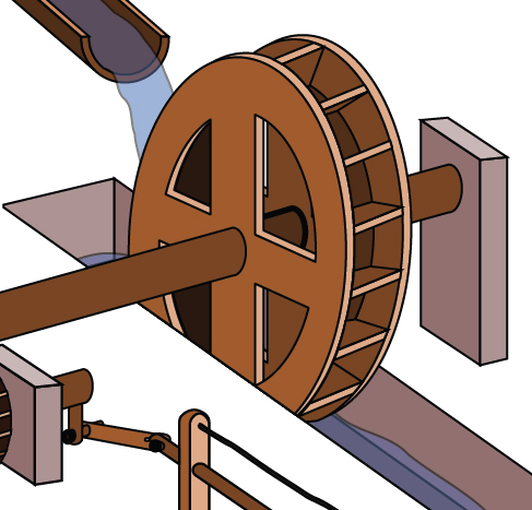
Figure 4.1.54:
Solution (click to reveal)
The wheel completes 1 rotation, or passes through an angle of \(2\pi\) radians in 5 seconds, so the angular speed would be \(\omega = \frac{2\pi}{5} \approx 1.257\) radians per second.