3.4 Graphs of Logarithmic Functions

NoteLearning Objectives

In this section, you will:

• Identify the domain of a logarithmic function.
• Graph logarithmic functions.

In Graphs of Exponential Functions, we saw how creating a graphical representation of an exponential model gives us another layer of insight for predicting future events. How do logarithmic graphs give us insight into situations? Because every logarithmic function is the inverse function of an exponential function, we can think of every output on a logarithmic graph as the input for the corresponding inverse exponential equation. In other words, logarithms give the cause for an effect.

To illustrate, suppose we invest \(\text{\$}2500\) in an account that offers an annual interest rate of \(5\%,\) compounded continuously. We already know that the balance in our account for any year \(t\) can be found with the equation \(A = 2500e^{0.05t}.\)

But what if we wanted to know the year for any balance? We would need to create a corresponding new function by interchanging the input and the output; thus we would need to create a logarithmic model for this situation. By graphing the model, we can see the output (year) for any input (account balance). For instance, what if we wanted to know how many years it would take for our initial investment to double? Figure 3.4.1 shows this point on the logarithmic graph.

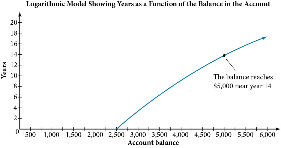
Figure 3.4.1:

In this section we will discuss the values for which a logarithmic function is defined, and then turn our attention to graphing the family of logarithmic functions.

3.4.1 Finding the Domain of a Logarithmic Function

Before working with graphs, we will take a look at the domain (the set of input values) for which the logarithmic function is defined.

Recall that the exponential function is defined as \(y = b^{x}\) for any real number \(x\) and constant \(b > 0,\) \(b \neq 1,\) where

• The domain of \(y\) is \(\left( {- \infty,\infty} \right).\)
• The range of \(y\) is \(\left( {0,\infty} \right).\)

In the last section we learned that the logarithmic function \(y = \log_{b}(x)\) is the inverse of the exponential function \(y = b^{x}.\) So, as inverse functions:

• The domain of \(y = \log_{b}(x)\) is the range of \(y = b^{x}:\) \(\left( {0,\infty} \right).\)
• The range of \(y = \log_{b}(x)\) is the domain of \(y = b^{x}:\) \(\left( {- \infty,\infty} \right).\)

Transformations of the parent function \(y = \log_{b}(x)\) behave similarly to those of other functions. Just as with other parent functions, we can apply the four types of transformations—shifts, stretches, compressions, and reflections.

In Graphs of Exponential Functions we saw that certain transformations can change the range of \(y = b^{x}.\) Similarly, applying transformations to the parent function \(y = \log_{b}(x)\) can change the domain. When finding the domain of a logarithmic function, therefore, it is important to remember that the domain consists only of positive real numbers. That is, the argument of the logarithmic function must be greater than zero.

For example, consider \(f(x) = \log_{4}\left( {2x - 3} \right).\) This function is defined for any values of \(x\) such that the argument, in this case \(2x - 3,\) is greater than zero. To find the domain, we set up an inequality and solve for \(x:\)

\[\begin{array}{ll} {2x - 3 > 0} & {\text{Show~the~argument~greater~than~zero}.} \\ {\mspace{9mu}\mspace{9mu}\mspace{9mu}\mspace{9mu}\mspace{9mu}\mspace{9mu}\mspace{9mu}\mspace{9mu}\mspace{9mu}\mspace{9mu} 2x > 3} & {\text{Add~3}.} \\ {\mspace{9mu}\mspace{9mu}\mspace{9mu}\mspace{9mu}\mspace{9mu}\mspace{9mu}\mspace{9mu}\mspace{9mu}\mspace{9mu}\mspace{9mu}\mspace{9mu}\mspace{9mu}\mspace{9mu} x > 1.5\begin{array}{llll} & & & \end{array}} & {\text{Divide~by~2}.} \end{array}\]

In interval notation, the domain of \(f(x) = \log_{4}\left( {2x - 3} \right)\) is \(\left( {1.5,\infty} \right).\)

ImportantHow To 3.4.2

Given a logarithmic function, identify the domain.

1. Set up an inequality showing the argument greater than zero.
2. Solve for \(x.\)
3. Write the domain in interval notation.

TipExample 3.4.3 — Identifying the Domain of a Logarithmic Shift

What is the domain of \(f(x) = \log_{2}(x + 3)?\)

Solution (click to reveal)

The logarithmic function is defined only when the input is positive, so this function is defined when \(x + 3 > 0.\) Solving this inequality,

\[\begin{array}{ll} {x + 3 > 0} & {\text{The~input~must~be~positive}.} \\ {x > - 3\begin{array}{llll} & & & \end{array}} & {\text{Subtract~3}.} \end{array}\]

The domain of \(f(x) = \log_{2}(x + 3)\) is \(\left( {- 3,\infty} \right).\)

WarningTry It 3.4.4

What is the domain of \(f(x) = \log_{5}(x - 2) + 1?\)

Solution (click to reveal)

\(\left( {2,\infty} \right)\)

TipExample 3.4.5 — Identifying the Domain of a Logarithmic Shift and Reflection

What is the domain of \(f(x) = \log(5 - 2x)?\)

Solution (click to reveal)

The logarithmic function is defined only when the input is positive, so this function is defined when \(5–2x > 0.\) Solving this inequality,

\[\begin{array}{ll} {5 - 2x > 0} & {\text{The~input~must~be~positive}.} \\ {- 2x > - 5} & {\text{Subtract~}5.} \\ {x < \frac{5}{2}\begin{array}{llll} & & & \end{array}} & {\text{Divide~by~} - 2\mspace{9mu}\text{and~switch~the~inequality}.} \end{array}\]

The domain of \(f(x) = \log(5 - 2x)\) is \(\left( {–\infty,\frac{5}{2}} \right).\)

WarningTry It 3.4.6

What is the domain of \(f(x) = \log(x - 5) + 2?\)

Solution (click to reveal)

\(\left( {5,\infty} \right)\)

3.4.2 Graphing Logarithmic Functions

Now that we have a feel for the set of values for which a logarithmic function is defined, we move on to graphing logarithmic functions. The family of logarithmic functions includes the parent function \(y = \log_{b}(x)\) along with all its transformations: shifts, stretches, compressions, and reflections.

We begin with the parent function \(y = \log_{b}(x).\) Because every logarithmic function of this form is the inverse of an exponential function with the form \(y = b^{x},\) their graphs will be reflections of each other across the line \(y = x.\) To illustrate this, we can observe the relationship between the input and output values of \(y = 2^{x}\) and its equivalent \(x = \log_{2}(y)\) in Table 3.4.7.

\(x\)	\(- 3\)	\(- 2\)	\(- 1\)	\(0\)	\(1\)	\(2\)	\(3\)
\(2^{x} = y\)	\(\frac{1}{8}\)	\(\frac{1}{4}\)	\(\frac{1}{2}\)	\(1\)	\(2\)	\(4\)	\(8\)
\(\log_{2}(y) = x\)	\(- 3\)	\(- 2\)	\(- 1\)	\(0\)	\(1\)	\(2\)	\(3\)

Table 3.4.7:

Using the inputs and outputs from Table 3.4.7, we can build another table to observe the relationship between points on the graphs of the inverse functions \(f(x) = 2^{x}\) and \(g(x) = \log_{2}(x).\) See Table 3.4.8.

\(f(x) = 2^{x}\)	\(\left( {- 3,\frac{1}{8}} \right)\)	\(\left( {- 2,\frac{1}{4}} \right)\)	\(\left( {- 1,\frac{1}{2}} \right)\)	\(\left( {0,1} \right)\) | \(\left( {1,2} \right)\) | \(\left( {2,4} \right)\) | \(\left( {3,8} \right)\) |
\(g(x) = \log_{2}(x)\)	\(\left( {\frac{1}{8}, - 3} \right)\)	\(\left( {\frac{1}{4}, - 2} \right)\)	\(\left( {\frac{1}{2}, - 1} \right)\)	\(\left( {1,0} \right)\) | \(\left( {2,1} \right)\) | \(\left( {4,2} \right)\) | \(\left( {8,3} \right)\) |

Table 3.4.8:

As we’d expect, the \(x\)- and \(y\)-coordinates are reversed for the inverse functions. Figure 3.4.9 shows the graph of \(f\) and \(g.\)

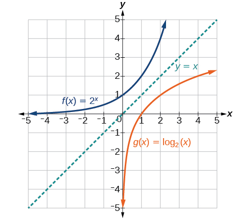
Figure 3.4.9: Notice that the graphs of \(f(x) = 2^{x}\) and \(g(x) = \log_{2}(x)\) are reflections about the line \(y = x.\)

Observe the following from the graph:

• \(f(x) = 2^{x}\) has a \(y\)-intercept at \((0,1)\) and \(g(x) = \log_{2}(x)\) has an \(x\)- intercept at \((1,0).\)
• The domain of \(f(x) = 2^{x},\) \(\left( {- \infty,\infty} \right),\) is the same as the range of \(g(x) = \log_{2}(x).\)
• The range of \(f(x) = 2^{x},\) \(\left( {0,\infty} \right),\) is the same as the domain of \(g(x) = \log_{2}(x).\)

NoteDefinition 3.4.10 — Characteristics of the Graph of the Parent Function, \(f(x) = \log_{b}(x):\)

For any real number \(x\) and constant \(b > 0,\) \(b \neq 1,\) we can see the following characteristics in the graph of \(f(x) = \log_{b}(x):\)

• one-to-one function
• vertical asymptote: \(x = 0\)
• domain: \((0,\infty)\)
• range: \(\left( {- \infty,\infty} \right)\)
• \(x\)-intercept: \((1,0)\) and key point \((b,1)\)
• \(y\)-intercept: none
• increasing if \(b > 1\)
• decreasing if \(0 < b < 1\)

See Figure 3.4.11.

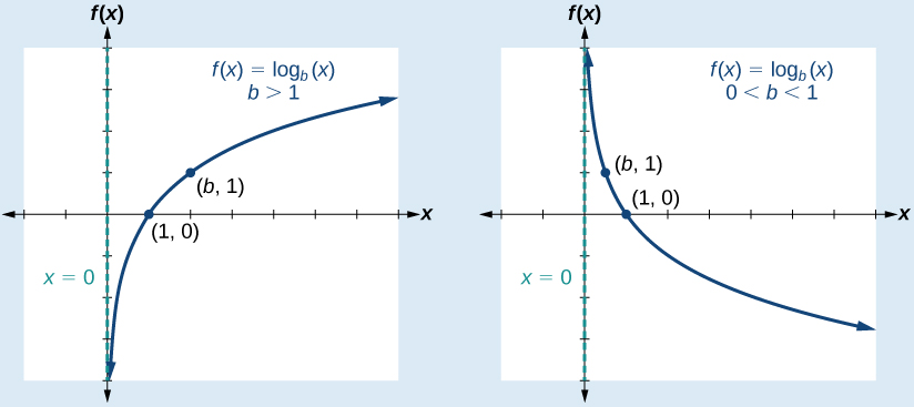
Figure 3.4.11:

Figure 3.4.12 shows how changing the base \(b\) in \(f(x) = \log_{b}(x)\) can affect the graphs. Observe that the graphs compress vertically as the value of the base increases. (Note: recall that the function \(\ln(x)\) has base \(e \approx \text{2}.\text{718.)}\)

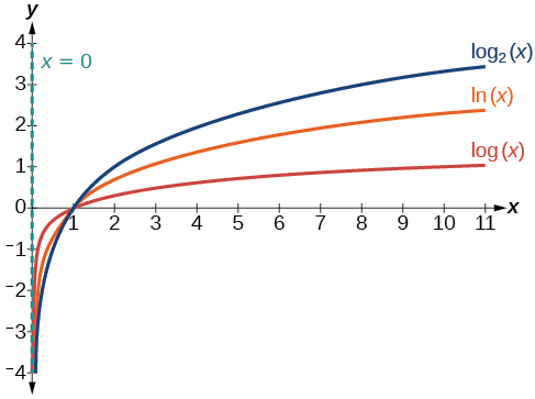
Figure 3.4.12: The graphs of three logarithmic functions with different bases, all greater than 1.

ImportantHow To 3.4.13

Given a logarithmic function with the form \(f(x) = \log_{b}(x),\) graph the function.

1. Draw and label the vertical asymptote, \(x = 0.\)
2. Plot the \(x\)-intercept, \(\left( {1,0} \right).\)
3. Plot the key point \(\left( {b,1} \right).\)
4. Draw a smooth curve through the points.
5. State the domain, \(\left( {0,\infty} \right),\) the range, \(\left( {- \infty,\infty} \right),\) and the vertical asymptote, \(x = 0.\)

TipExample 3.4.14 — Graphing a Logarithmic Function with the Form \(f\)(\(x\)) = log\(b\)(\(x\)).

Graph \(f(x) = \log_{5}(x).\) State the domain, range, and asymptote.

Solution (click to reveal)

Before graphing, identify the behavior and key points for the graph.

• Since \(b = 5\) is greater than one, we know the function is increasing. The left tail of the graph will approach the vertical asymptote \(x = 0,\) and the right tail will increase slowly without bound.
• The \(x\)-intercept is \(\left( {1,0} \right).\)
• The key point \(\left( {5,1} \right)\) is on the graph.
• We draw and label the asymptote, plot and label the points, and draw a smooth curve through the points (see Figure 3.4.16).

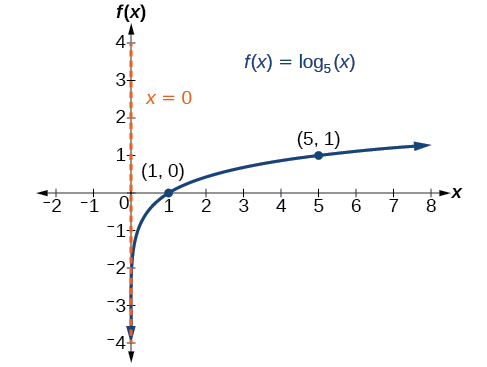
Figure 5

The domain is \(\left( {0,\infty} \right),\) the range is \(\left( {- \infty,\infty} \right),\) and the vertical asymptote is \(x = 0.\)

WarningTry It 3.4.15

Graph \(f(x) = \log_{\frac{1}{5}}(x).\) State the domain, range, and asymptote.

Solution (click to reveal)

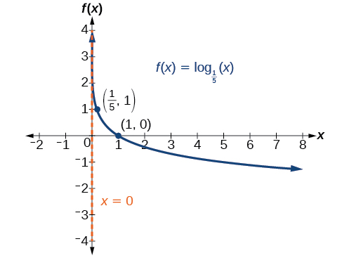
The domain is \(\left( {0,\infty} \right),\) the range is \(\left( {- \infty,\infty} \right),\) and the vertical asymptote is \(x = 0.\)

3.4.3 Graphing Transformations of Logarithmic Functions

As we mentioned in the beginning of the section, transformations of logarithmic graphs behave similarly to those of other parent functions. We can shift, stretch, compress, and reflect the parent function \(y = \log_{b}(x)\) without loss of shape.

Graphing a Horizontal Shift of \(f\)(\(x\)) = log\(b\)(\(x\))

When a constant \(c\) is added to the input of the parent function \(f(x) = log_{b}(x),\) the result is a horizontal shift \(c\) units in the opposite direction of the sign on \(c.\) To visualize horizontal shifts, we can observe the general graph of the parent function \(f(x) = \log_{b}(x)\) and for \(c > 0\) alongside the shift left, \(g(x) = \log_{b}\left( {x + c} \right),\) and the shift right, \(h(x) = \log_{b}\left( {x - c} \right).\) See Figure 3.4.16.

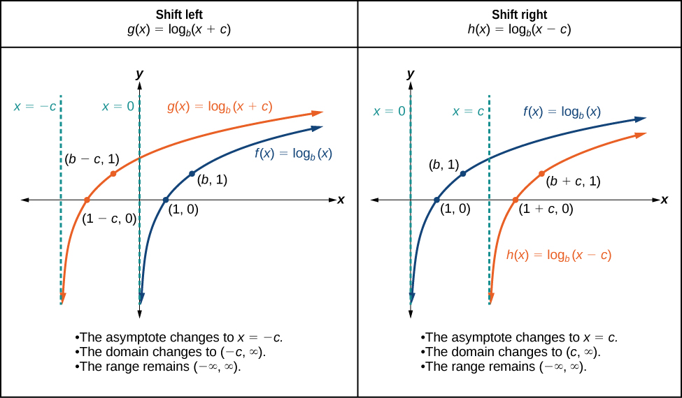
Figure 3.4.16:

NoteDefinition 3.4.17 — Horizontal Shifts of the Parent Function \(f(x) = \log_{b}(x)\)

For any constant \(c,\) the function \(f(x) = \log_{b}\left( {x + c} \right)\)

• shifts the parent function \(y = \log_{b}(x)\) left \(c\) units if \(c > 0.\)
• shifts the parent function \(y = \log_{b}(x)\) right \(c\) units if \(c < 0.\)
• has the vertical asymptote \(x = - c.\)
• has domain \(\left( {- c,\infty} \right).\)
• has range \(\left( {- \infty,\infty} \right).\)

ImportantHow To 3.4.18

Given a logarithmic function with the form \(f(x) = \log_{b}\left( {x + c} \right),\) graph the translation.

1. Identify the horizontal shift:
   

2. If \(c > 0,\) shift the graph of \(f(x) = \log_{b}(x)\) left \(c\) units.
   

3. If \(c < 0,\) shift the graph of \(f(x) = \log_{b}(x)\) right \(c\) units.

4. Draw the vertical asymptote \(x = - c.\)

5. Identify three key points from the parent function. Find new coordinates for the shifted functions by subtracting \(c\) from the \(x\) coordinate.

6. Label the three points.

7. The Domain is \(\left( {- c,\infty} \right),\) the range is \(\left( {- \infty,\infty} \right),\) and the vertical asymptote is \(x = - c.\)

TipExample 3.4.19 — Graphing a Horizontal Shift of the Parent Function \(y\) = log\(b\)(\(x\))

Sketch the horizontal shift \(f(x) = \log_{3}(x - 2)\) alongside its parent function. Include the key points and asymptotes on the graph. State the domain, range, and asymptote.

Solution (click to reveal)

Since the function is \(f(x) = \log_{3}(x - 2),\) we notice \(x + \left( {- 2} \right) = x–2.\)

Thus \(c = - 2,\) so \(c < 0.\) This means we will shift the function \(f(x) = \log_{3}(x)\) right 2 units.

The vertical asymptote is \(x = - ( - 2)\) or \(x = 2.\)

Consider the three key points from the parent function, \(\left( {\frac{1}{3},-1} \right),\) \(\left( {1,0} \right),\) and \(\left( {3,1} \right).\)

The new coordinates are found by adding 2 to the \(x\) coordinates.

Label the points \(\left( {\frac{7}{3},-1} \right),\) \(\left( {3,0} \right),\) and \(\left( {5,1} \right).\)

The domain is \(\left( {2,\infty} \right),\) the range is \(\left( {- \infty,\infty} \right),\) and the vertical asymptote is \(x = 2.\)

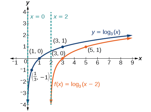
Figure 7

WarningTry It 3.4.20

Sketch a graph of \(f(x) = \log_{3}(x + 4)\) alongside its parent function. Include the key points and asymptotes on the graph. State the domain, range, and asymptote.

Solution (click to reveal)

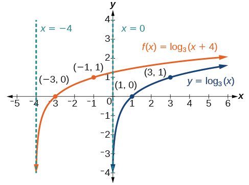
The domain is \(\left( {- 4,\infty} \right),\) the range \(\left( {- \infty,\infty} \right),\) and the asymptote \(x = –4.\)

Graphing a Vertical Shift of \(f\)(\(x\)) = log\(b\)(\(x\))

When a constant \(d\) is added to the parent function \(f(x) = \log_{b}(x),\) the result is a vertical shift \(d\) units in the direction of the sign on \(d.\) To visualize vertical shifts, we can observe the general graph of the parent function \(f(x) = \log_{b}(x)\) alongside the shift up, \(g(x) = \log_{b}(x) + d\) and the shift down, \(h(x) = \log_{b}(x) - d.\) See Figure 3.4.21.

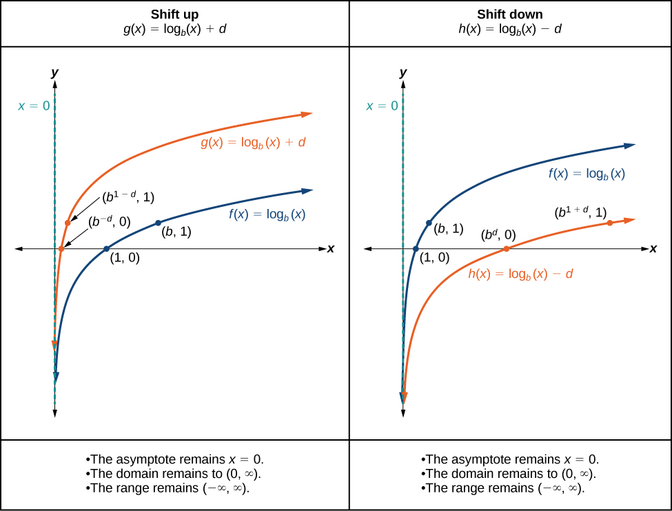
Figure 3.4.21:

NoteDefinition 3.4.22 — Vertical Shifts of the Parent Function \(y = \log_{b}(x)\)

For any constant \(d,\) the function \(f(x) = \log_{b}(x) + d\)

• shifts the parent function \(y = \log_{b}(x)\) up \(d\) units if \(d > 0.\)
• shifts the parent function \(y = \log_{b}(x)\) down \(d\) units if \(d < 0.\)
• has the vertical asymptote \(x = 0.\)
• has domain \(\left( {0,\infty} \right).\)
• has range \(\left( {- \infty,\infty} \right).\)

ImportantHow To 3.4.23

Given a logarithmic function with the form \(f(x) = \log_{b}(x) + d,\) graph the translation.

1. Identify the vertical shift:
   

• If \(d > 0,\) shift the graph of \(f(x) = \log_{b}(x)\) up \(d\) units.
  
• If \(d < 0,\) shift the graph of \(f(x) = \log_{b}(x)\) down \(d\) units.

2. Draw the vertical asymptote \(x = 0.\)

3. Identify three key points from the parent function. Find new coordinates for the shifted functions by adding \(d\) to the \(y\) coordinate.

4. Label the three points.

5. The domain is \(\left( {0,\infty} \right),\) the range is \(\left( {- \infty,\infty} \right),\) and the vertical asymptote is \(x = 0.\)

TipExample 3.4.24 — Graphing a Vertical Shift of the Parent Function \(f\)(\(x\)) = log\(b\)(\(x\))

Sketch a graph of \(f(x) = \log_{3}(x) - 2\) alongside its parent function. Include the key points and asymptote on the graph. State the domain, range, and asymptote.

Solution (click to reveal)

Since the function is \(f(x) = \log_{3}(x) - 2,\) we will notice \(d = –2.\) Thus \(d < 0.\)

This means we will shift the function \(f(x) = \log_{3}(x)\) down 2 units.

The vertical asymptote is \(x = 0.\)

Consider the three key points from the parent function, \(\left( {\frac{1}{3},-1} \right),\) \(\left( {1,0} \right),\) and \(\left( {3,1} \right).\)

The new coordinates are found by subtracting 2 from the y coordinates.

Label the points \(\left( {\frac{1}{3},-3} \right),\) \(\left( {1,-2} \right),\) and \(\left( {3,-1} \right).\)

The domain is \(\left( {0,\infty} \right),\) the range is \(\left( {- \infty,\infty} \right),\) and the vertical asymptote is \(x = 0.\)

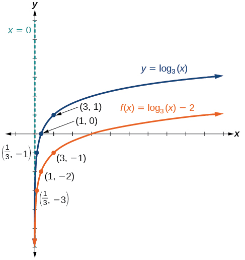
Figure 9

The domain is \(\left( {0,\infty} \right),\) the range is \(\left( {- \infty,\infty} \right),\) and the vertical asymptote is \(x = 0.\)

WarningTry It 3.4.25

Sketch a graph of \(f(x) = \log_{2}(x) + 2\) alongside its parent function. Include the key points and asymptote on the graph. State the domain, range, and asymptote.

Solution (click to reveal)

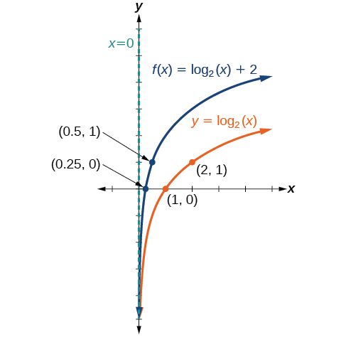
The domain is \(\left( {0,\infty} \right),\) the range is \(\left( {- \infty,\infty} \right),\) and the vertical asymptote is \(x = 0.\)

Graphing Stretches and Compressions of \(f\)(\(x\)) = log\(b\)(\(x\))

When the parent function \(f(x) = \log_{b}(x)\) is multiplied by a constant \(a > 0,\) the result is a vertical stretch or compression of the original graph. To visualize stretches and compressions, we set \(a > 1\) and observe the general graph of the parent function \(f(x) = \log_{b}(x)\) alongside the vertical stretch, \(g(x) = a\log_{b}(x)\) and the vertical compression, \(h(x) = \frac{1}{a}\log_{b}(x).\) See Figure 3.4.26.

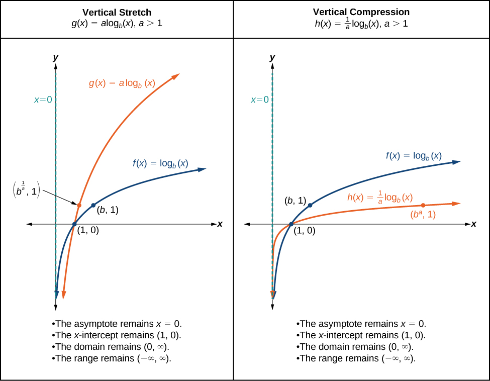
Figure 3.4.26:

NoteDefinition 3.4.27 — Vertical Stretches and Compressions of the Parent Function \(y = \log_{b}(x)\)

For any constant \(a > 1,\) the function \(f(x) = a\log_{b}(x)\)

• stretches the parent function \(y = \log_{b}(x)\) vertically by a factor of \(a\) if \(a > 1.\)
• compresses the parent function \(y = \log_{b}(x)\) vertically by a factor of \(a\) if \(0 < a < 1.\)
• has the vertical asymptote \(x = 0.\)
• has the \(x\)-intercept \(\left( {1,0} \right).\)
• has domain \(\left( {0,\infty} \right).\)
• has range \(\left( {- \infty,\infty} \right).\)

ImportantHow To 3.4.28

Given a logarithmic function with the form \(f(x) = a\log_{b}(x),\) \(a > 0,\) graph the translation.

1. Identify the vertical stretch or compressions:
   

• If \(\left| a \middle| > 1, \right.\) the graph of \(f(x) = \log_{b}(x)\) is stretched by a factor of \(a\) units.
  
• If \(\left| a \middle| < 1, \right.\) the graph of \(f(x) = \log_{b}(x)\) is compressed by a factor of \(a\) units.

2. Draw the vertical asymptote \(x = 0.\)

3. Identify three key points from the parent function. Find new coordinates for the shifted functions by multiplying the \(y\) coordinates by \(a.\)

4. Label the three points.

5. The domain is \(\left( {0,\infty} \right),\) the range is \(\left( {- \infty,\infty} \right),\) and the vertical asymptote is \(x = 0.\)

TipExample 3.4.29 — Graphing a Stretch or Compression of the Parent Function \(f\)(\(x\)) = log\(b\)(\(x\))

Sketch a graph of \(f(x) = 2\log_{4}(x)\) alongside its parent function. Include the key points and asymptote on the graph. State the domain, range, and asymptote.

Solution (click to reveal)

Since the function is \(f(x) = 2\log_{4}(x),\) we will notice \(a = 2.\)

This means we will stretch the function \(f(x) = \log_{4}(x)\) by a factor of 2.

The vertical asymptote is \(x = 0.\)

Consider the three key points from the parent function, \(\left( {\frac{1}{4},-1} \right),\) \(\left( {1,0}\operatorname{),} \right.\) and \(\left( {4,1} \right).\)

The new coordinates are found by multiplying the \(y\) coordinates by 2.

Label the points \(\left( {\frac{1}{4},-2} \right),\) \(\left( {1,0} \right)\mspace{9mu},\) and \(\left( {4,\text{2}} \right).\)

The domain is \(\left( {0,\mspace{9mu}\infty} \right),\) the range is \(\left( {-\infty,\infty}\operatorname{),} \right.\) and the vertical asymptote is \(x = 0.\) See Figure 3.4.33.

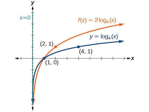
Figure 11

The domain is \(\left( {0,\infty} \right),\) the range is \(\left( {- \infty,\infty} \right),\) and the vertical asymptote is \(x = 0.\)

WarningTry It 3.4.30

Sketch a graph of \(f(x) = \frac{1}{2}\mspace{9mu}\log_{4}(x)\) alongside its parent function. Include the key points and asymptote on the graph. State the domain, range, and asymptote.

Solution (click to reveal)

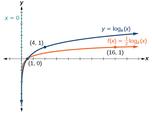
The domain is \(\left( {0,\infty} \right),\) the range is \(\left( {- \infty,\infty} \right),\) and the vertical asymptote is \(x = 0.\)

TipExample 3.4.31 — Combining a Shift and a Stretch

Sketch a graph of \(f(x) = 5\log(x + 2).\) State the domain, range, and asymptote.

Solution (click to reveal)

Remember: what happens inside parentheses happens first. First, we move the graph left 2 units, then stretch the function vertically by a factor of 5, as in Figure 3.4.33. The vertical asymptote will be shifted to \(x = -2.\) The \(x\)-intercept will be \((-1,0).\) The domain will be \(\left( {-2,\infty} \right).\) Two points will help give the shape of the graph: \((-1,0)\) and \((8,5\operatorname{).}\) We chose \(x = 8\) as the \(x\)-coordinate of one point to graph because when \(x = 8,\) \(x + 2 = 10,\) the base of the common logarithm.

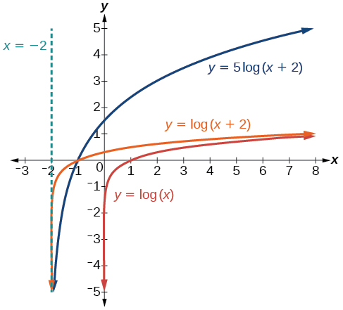
Figure 12

The domain is \(\left( {- 2,\infty} \right),\) the range is \(\left( {- \infty,\infty} \right),\) and the vertical asymptote is \(x = - 2.\)

WarningTry It 3.4.32

Sketch a graph of the function \(f(x) = 3\log(x - 2) + 1.\) State the domain, range, and asymptote.

Solution (click to reveal)

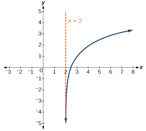
The domain is \(\left( {2,\infty} \right),\) the range is \(\left( {- \infty,\infty} \right),\) and the vertical asymptote is \(x = 2.\)

Graphing Reflections of \(f\)(\(x\)) = log\(b\)(\(x\))

When the parent function \(f(x) = \log_{b}(x)\) is multiplied by \(-1,\) the result is a reflection about the \(x\)-axis. When the input is multiplied by \(-1,\) the result is a reflection about the \(y\)-axis. To visualize reflections, we restrict \(b > 1,\) and observe the general graph of the parent function \(f(x) = \log_{b}(x)\) alongside the reflection about the \(x\)-axis, \(g(x) = {-log}_{b}(x)\) and the reflection about the \(y\)-axis, \(h(x) = \log_{b}\left( {- x} \right).\)

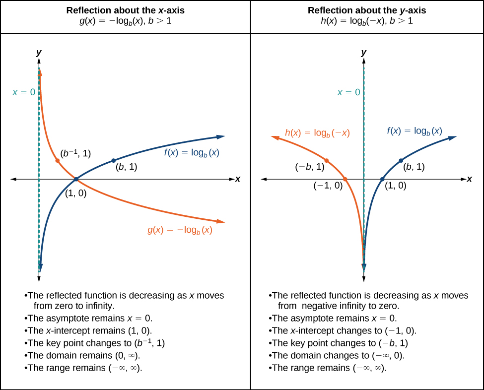
Figure 3.4.33:

NoteDefinition 3.4.34 — Reflections of the Parent Function \(y = \log_{b}(x)\)

The function \(f(x) = {-log}_{b}(x)\)

• reflects the parent function \(y = \log_{b}(x)\) about the \(x\)-axis.
• has domain, \(\left( {0,\infty} \right),\) range, \(\left( {- \infty,\infty} \right),\) and vertical asymptote, \(x = 0,\) which are unchanged from the parent function.

The function \(f(x) = \log_{b}\left( {- x} \right)\)

• reflects the parent function \(y = \log_{b}(x)\) about the \(y\)-axis.
• has domain \(\left( {- \infty,0} \right).\)
• has range, \(\left( {- \infty,\infty} \right),\) and vertical asymptote, \(x = 0,\) which are unchanged from the parent function.

ImportantHow To 3.4.35

Given a logarithmic function with the parent function \(f(x) = \log_{b}(x),\) graph a translation.

\(\text{If~}f(x) = - \log_{b}(x)\)	\(\text{If~}f(x) = \log_{b}( - x)\)
Draw the vertical asymptote, \(x = 0.\)	Draw the vertical asymptote, \(x = 0.\)
Plot the \(x\)-intercept, \(\left( {1,0} \right).\) | 2. Plot the \(x\)-intercept, \(\left( {1,0} \right).\) |
Reflect the graph of the parent function \(f(x) = \log_{b}(x)\) about the \(x\)-axis.	Reflect the graph of the parent function \(f(x) = \log_{b}(x)\) about the \(y\)-axis.
Draw a smooth curve through the points.	Draw a smooth curve through the points.
State the domain, (0, ∞), the range, (−∞, ∞), and the vertical asymptote \(x = 0\).	State the domain, (−∞, 0) the range, (−∞, ∞) and the vertical asymptote \(x = 0.\)

Table 3.4.36:

TipExample 3.4.37 — Graphing a Reflection of a Logarithmic Function

Sketch a graph of \(f(x) = \log( - x)\) alongside its parent function. Include the key points and asymptote on the graph. State the domain, range, and asymptote.

Solution (click to reveal)

Before graphing \(f(x) = \log( - x),\) identify the behavior and key points for the graph.

• Since \(b = 10\) is greater than one, we know that the parent function is increasing. Since the input value is multiplied by \(-1,\) \(f\) is a reflection of the parent graph about the \(y\)-axis. Thus, \(f(x) = \log( - x)\) will be decreasing as \(x\) moves from negative infinity to zero, and the right tail of the graph will approach the vertical asymptote \(x = 0.\)
• The \(x\)-intercept is \(\left( {-1,0} \right).\)
• We draw and label the asymptote, plot and label the points, and draw a smooth curve through the points.

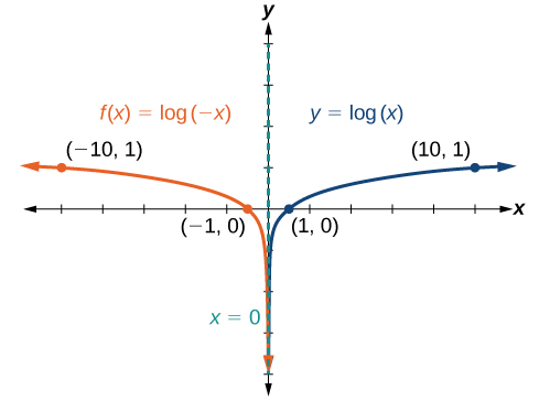
Figure 14

The domain is \(\left( {- \infty,0} \right),\) the range is \(\left( {- \infty,\infty} \right),\) and the vertical asymptote is \(x = 0.\)

WarningTry It 3.4.38

Graph \(f(x) = - \log( - x).\) State the domain, range, and asymptote.

Solution (click to reveal)

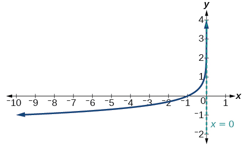
The domain is \(\left( {- \infty,0} \right),\) the range is \(\left( {- \infty,\infty} \right),\) and the vertical asymptote is \(x = 0.\)

ImportantHow To 3.4.39

Given a logarithmic equation, use a graphing calculator to approximate solutions.

1. Press [Y=]. Enter the given logarithm equation or equations as Y1= and, if needed, Y2=.
2. Press [GRAPH] to observe the graphs of the curves and use [WINDOW] to find an appropriate view of the graphs, including their point(s) of intersection.
3. To find the value of \(x,\) we compute the point of intersection. Press [2ND] then [CALC]. Select “intersect” and press [ENTER] three times. The point of intersection gives the value of \(x,\) for the point(s) of intersection.

TipExample 3.4.40 — Approximating the Solution of a Logarithmic Equation

Solve \(4\ln(x) + 1 = - 2\ln\left( {x - 1} \right)\) graphically. Round to the nearest thousandth.

Solution (click to reveal)

Press [Y=] and enter \(4\ln(x) + 1\) next to Y1=. Then enter \(- 2\ln\left( {x - 1} \right)\) next to Y2=. For a window, use the values 0 to 5 for \(x\) and –10 to 10 for \(y.\) Press [GRAPH]. The graphs should intersect somewhere a little to right of \(x = 1.\)

For a better approximation, press [2ND] then [CALC]. Select [5: intersect] and press [ENTER] three times. The \(x\)-coordinate of the point of intersection is displayed as 1.3385297. (Your answer may be different if you use a different window or use a different value for Guess?) So, to the nearest thousandth, \(x \approx 1.339.\)

WarningTry It 3.4.41

Solve \(5\log\left( {x + 2} \right) = 4 - \log(x)\) graphically. Round to the nearest thousandth.

Solution (click to reveal)

\(x \approx 3.049\)

Summarizing Translations of the Logarithmic Function

Now that we have worked with each type of translation for the logarithmic function, we can summarize each in Table 3.4.42 to arrive at the general equation for translating exponential functions.

Transformations of the Parent Function \(y = \log_{b}(x)\)
Transformation	Form
Shift Horizontally \(c\) units to the left Vertically \(d\) units up	\(y = \log_{b}\left( {x + c} \right) + d\)
Stretch and Compress Stretch if \(|a| > 1\) Compression if \(|a| < 1\)	\(y = a\log_{b}(x)\)
Reflect about the \(x\)-axis	\(y = - \log_{b}(x)\)
Reflect about the \(y\)-axis	\(y = \log_{b}\left( {- x} \right)\)
General equation for all translations	\(y = a\log_{b}(x + c) + d\)

Table 3.4.42:

NoteDefinition 3.4.43 — Transformations of Logarithmic Functions

All transformations of the parent logarithmic function, \(y = \log_{b}(x),\) have the form

\[~f(x) = a\log_{b}\left( {x + c} \right) + d\]

where the parent function, \(y = \log_{b}(x),b > 1,\) is

• shifted vertically up \(d\) units.
• shifted horizontally to the left \(c\) units.
• stretched vertically by a factor of \(|a|\) if \(|a| > 0.\)
• compressed vertically by a factor of \(|a|\) if \(0 < |a| < 1.\)
• reflected about the \(x\)-axis when \(a < 0.\)

For \(f(x) = \log\left( {- x} \right),\) the graph of the parent function is reflected about the \(y\)-axis.

TipExample 3.4.44 — Finding the Vertical Asymptote of a Logarithm Graph

What is the vertical asymptote of \(f(x) = -2\log_{3}(x + 4) + 5?\)

Solution (click to reveal)

The vertical asymptote is at \(x = - 4.\)

The coefficient, the base, and the upward translation do not affect the asymptote. The shift of the curve 4 units to the left shifts the vertical asymptote to \(x = -4.\)

WarningTry It 3.4.45

What is the vertical asymptote of \(f(x) = 3 + \ln(x - 1)?\)

Solution (click to reveal)

\(x = 1\)

TipExample 3.4.46 — Finding the Equation from a Graph

Find a possible equation for the common logarithmic function graphed in Figure 3.4.47.

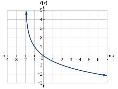
Figure 3.4.47:

Solution (click to reveal)

This graph has a vertical asymptote at \(x = –2\) and has been vertically reflected. We do not know yet the vertical shift or the vertical stretch. We know so far that the equation will have form:

\[f(x) = - a\log(x + 2) + k\]

It appears the graph passes through the points \(\left( {–1,1} \right)\) and \(\left( {2,–1} \right).\) Substituting \(\left( {–1,1} \right),\)

\[\begin{array}{ll} {1 = - a\log(-1 + 2) + k\mspace{9mu}\mspace{9mu}\mspace{9mu}\mspace{9mu}\mspace{9mu}\mspace{9mu}\mspace{9mu}\mspace{9mu}\mspace{9mu}\mspace{9mu}\mspace{9mu}\mspace{9mu}} & {\text{Substitute~}(-1,1).} \\ {1 = - a\log(1) + k} & {\text{Arithmetic}.} \\ {1 = k} & {\text{log(1)} = 0.} \end{array}\]

Next, substituting in \(\left( {2,–1} \right)\) ,

\[\begin{array}{lll} {- 1 = - a\log(2 + 2) + 1} & & {\text{Plug~in~}(2,-1).} \\ {- 2 = - a\log(4)} & & {\text{Arithmetic}.} \\ {\mspace{9mu}\ a = \frac{2}{\log(4)}} & & {\text{Solve~for~}a.} \end{array}\]

This gives us the equation \(f(x) = –\frac{2}{\log(4)}\log(x + 2) + 1.\)

We can verify this answer by comparing the function values in Table 3.4.48 with the points on the graph in Figure 3.4.47.

\(x\)	−1	0	1	2	3
\(f(x)\)	1	0	−0.58496	−1	−1.3219
\(x\)	4	5	6	7	8
\(f(x)\)	−1.5850	−1.8074	−2	−2.1699	−2.3219

Table 3.4.48:

WarningTry It 3.4.49

Give the equation of the natural logarithm graphed in Figure 3.4.50.

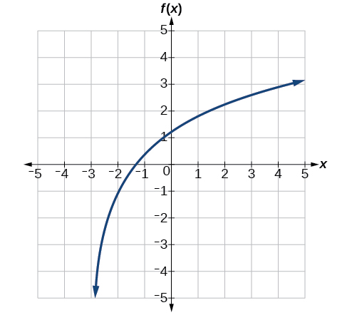
Figure 3.4.50:

Solution (click to reveal)

\(f(x) = 2\ln(x + 3) - 1\)

NoteQ&A 3.4.51

Is it possible to tell the domain and range and describe the end behavior of a function just by looking at the graph?

Yes, if we know the function is a general logarithmic function. For example, look at the graph in Figure 3.4.50. The graph approaches \(x = -3\) (or thereabouts) more and more closely, so \(x = -3\) is, or is very close to, the vertical asymptote. It approaches from the right, so the domain is all points to the right, \(\left\{ x\mspace{9mu} \middle| \mspace{9mu} x > -3 \right\}.\) The range, as with all general logarithmic functions, is all real numbers. And we can see the end behavior because the graph goes down as it goes left and up as it goes right. The end behavior is that as \(x\rightarrow - 3^{+},f(x)\rightarrow - \infty\) and as \(x\rightarrow\infty,f(x)\rightarrow\infty.\)