1.1 Functions and Function Notation

Learning Objectives

In this section, you will:

Determine whether a relation represents a function.
Find the value of a function.
Determine whether a function is one-to-one.
Use the vertical line test to identify functions.
Graph the functions listed in the library of functions.

A jetliner changes altitude as its distance from the starting point of a flight increases. The weight of a growing child increases with time. In each case, one quantity depends on another. There is a relationship between the two quantities that we can describe, analyze, and use to make predictions. In this section, we will analyze such relationships.

1.1.1 Determining Whether a Relation Represents a Function

A relation is a set of ordered pairs. The set of the first components of each ordered pair is called the domain and the set of the second components of each ordered pair is called the range. Consider the following set of ordered pairs. The first numbers in each pair are the first five natural numbers. The second number in each pair is twice that of the first.

\[\{(1,\mspace{9mu} 2),\mspace{9mu}(2,\mspace{9mu} 4),\mspace{9mu}(3,\mspace{9mu} 6),\mspace{9mu}(4,\mspace{9mu} 8),\mspace{9mu}(5,\mspace{9mu} 10)\}\]

The domain is $\{ 1,\mspace{9mu} 2,\mspace{9mu} 3,\mspace{9mu} 4,\mspace{9mu} 5\}.$ The range is $\{ 2,\mspace{9mu} 4,\mspace{9mu} 6,\mspace{9mu} 8,\mspace{9mu} 10\}.$

Note that each value in the domain is also known as an input value, or independent variable, and is often labeled with the lowercase letter $x.$ Each value in the range is also known as an output value, or dependent variable, and is often labeled lowercase letter $y.$

A function $f$ is a relation that assigns a single value in the range to each value in the domain. In other words, no $x$-values are repeated. For our example that relates the first five natural numbers to numbers double their values, this relation is a function because each element in the domain, $\{ 1,\mspace{9mu} 2,\mspace{9mu} 3,\mspace{9mu} 4,\mspace{9mu} 5\},$ is paired with exactly one element in the range, $\{ 2,\mspace{9mu} 4,\mspace{9mu} 6,\mspace{9mu} 8,\mspace{9mu} 10\}.$

Now let’s consider the set of ordered pairs that relates the terms “even” and “odd” to the first five natural numbers. It would appear as

\[\{{(\text{odd},\mspace{9mu} 1),\mspace{9mu}(\text{even},\mspace{9mu} 2),\mspace{9mu}(\text{odd},\mspace{9mu} 3),\mspace{9mu}(\text{even},\mspace{9mu} 4),\mspace{9mu}(\text{odd},\mspace{9mu} 5)}\}\]

Notice that each element in the domain, $\{\text{even,}\mspace{9mu}\text{odd}\}$ is not paired with exactly one element in the range, $\{ 1,\mspace{9mu} 2,\mspace{9mu} 3,\mspace{9mu} 4,\mspace{9mu} 5\}.$ For example, the term “odd” corresponds to three values from the range, $\{ 1,\mspace{9mu} 3,\mspace{9mu} 5\}$ and the term “even” corresponds to two values from the range, $\{ 2,\mspace{9mu} 4\}.$ This violates the definition of a function, so this relation is not a function.

Figure 1.1.1 compares relations that are functions and not functions.

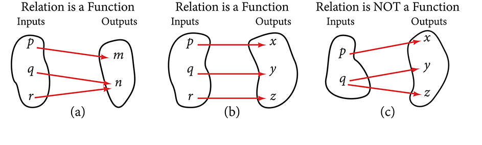
Three relations that demonstrate what constitute a function.

Figure 1.1.1: (a) This relationship is a function because each input is associated with a single output. Note that input $q$ and $r$ both give output $n.$ (b) This relationship is also a function. In this case, each input is associated with a single output. (c) This relationship is not a function because input $q$ is associated with two different outputs.

Definition 1.1.2 — Function

A function is a relation in which each possible input value leads to exactly one output value. We say “the output is a function of the input.”

The input values make up the domain, and the output values make up the range.

How To 1.1.3

Given a relationship between two quantities, determine whether the relationship is a function.

Identify the input values.
Identify the output values.
If each input value leads to only one output value, classify the relationship as a function. If any input value leads to two or more outputs, do not classify the relationship as a function.

Example 1.1.4 — Determining If Menu Price Lists Are Functions

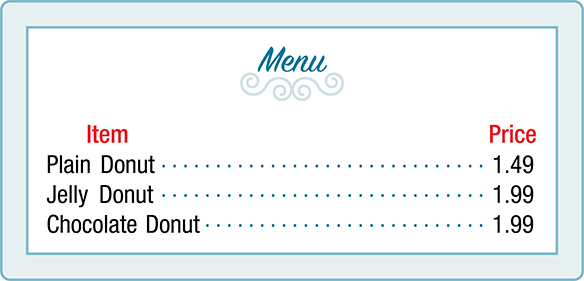
The coffee shop menu, shown below, consists of items and their prices.
ⓐ Is price a function of the item?
ⓑ Is the item a function of the price?

Solution (click to reveal)

ⓐ Let’s begin by considering the input as the items on the menu. The output values are then the prices.

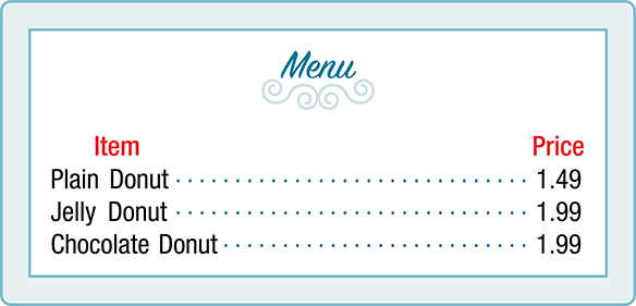
Each item on the menu has only one price, so the price is a function of the item.
ⓑ Two items on the menu have the same price. If we consider the prices to be the input values and the items to be the output, then the same input value could have more than one output associated with it. See the image below.

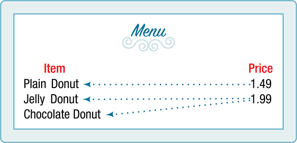
Therefore, the item is a not a function of price.

Example 1.1.5 — Determining If Class Grade Rules Are Functions

In a particular math class, the overall percent grade corresponds to a grade point average. Is grade point average a function of the percent grade? Is the percent grade a function of the grade point average? Table 1.1.6 shows a possible rule for assigning grade points.

Percent grade	0–56	57–61	62–66	67–71	72–77	78–86	87–91	92–100
Grade point average	0.0	1.0	1.5	2.0	2.5	3.0	3.5	4.0

Table 1.1.6:

Solution (click to reveal)

For any percent grade earned, there is an associated grade point average, so the grade point average is a function of the percent grade. In other words, if we input the percent grade, the output is a specific grade point average.

In the grading system given, there is a range of percent grades that correspond to the same grade point average. For example, students who receive a grade point average of 3.0 could have a variety of percent grades ranging from 78 all the way to 86. Thus, percent grade is not a function of grade point average.

Try It 1.1.7

Table 1.1.8 lists the five greatest baseball players of all time in order of rank.

Player	Rank
Babe Ruth	1
Willie Mays	2
Ty Cobb	3
Walter Johnson	4
Hank Aaron	5

Table 1.1.8:

ⓐ Is the rank a function of the player name?

ⓑ Is the player name a function of the rank?

Solution (click to reveal)

ⓐ yes

ⓑ yes (Note: If two players had been tied for, say, 4th place, then the name would not have been a function of rank.)

Using Function Notation

Once we determine that a relationship is a function, we need to display and define the functional relationships so that we can understand and use them, and sometimes also so that we can program them into computers. There are various ways of representing functions. A standard function notation is one representation that facilitates working with functions.

To represent “height is a function of age,” we start by identifying the descriptive variables $h$ for height and $a$ for age. The letters $f,\mspace{9mu} g,$ and $h$ are often used to represent functions just as we use $x,\mspace{9mu} y,$ and $z$ to represent numbers and $A,\mspace{9mu} B,$ and $C$ to represent sets.

\[\begin{array}{lllll} {h\mspace{9mu}\text{is~}f\mspace{9mu}\text{of~}a} & & & & {\text{We~name~the~function~}f;\mspace{9mu}\text{height~is~a~function~of~age}.} \\ {h = f(a)} & & & & {\text{We~use~parentheses~to~indicate~the~function~input}\text{.~}} \\ {f(a)} & & & & {\text{We~name~the~function~}f;\mspace{9mu}\text{the~expression~is~read~as~“}f\mspace{9mu}\text{of~}a\text{.”}} \end{array}\]

Remember, we can use any letter to name the function; the notation $h(a)$ shows us that $h$ depends on $a.$ The value $a$ must be put into the function $h$ to get a result. The parentheses indicate that age is input into the function; they do not indicate multiplication.

We can also give an algebraic expression as the input to a function. For example $f\left( {a + b} \right)$ means “first add $a$ and $b$, and the result is the input for the function $f$.” The operations must be performed in this order to obtain the correct result.

Definition 1.1.9 — Function Notation

The notation $y = f(x)$ defines a function named $f.$ This is read as $``y$ is a function of $x."$ The letter $x$ represents the input value, or independent variable. The letter $y\text{,}$ or $f(x),$ represents the output value, or dependent variable.

Example 1.1.10 — Using Function Notation for Days in a Month

Use function notation to represent a function whose input is the name of a month and output is the number of days in that month. Assume that the domain does not include leap years.

Solution (click to reveal)

The number of days in a month is a function of the name of the month, so if we name the function $f,$ we write $\text{days} = f(\text{month})$ or $d = f(m).$ The name of the month is the input to a “rule” that associates a specific number (the output) with each input.

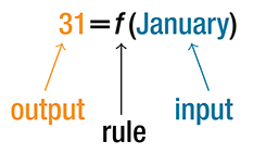
The function 31 = f(January) where 31 is the output, f is the rule, and January is the input.

Figure 2

For example, $f\left( \text{March} \right) = 31,$ because March has 31 days. The notation $d = f(m)$ reminds us that the number of days, $d$ (the output), is dependent on the name of the month, $m$ (the input).

Note that the inputs to a function do not have to be numbers; function inputs can be names of people, labels of geometric objects, or any other element that determines some kind of output. However, most of the functions we will work with in this book will have numbers as inputs and outputs.

Example 1.1.11 — Interpreting Function Notation

A function $N = f(y)$ gives the number of police officers, $N,$ in a town in year $y.$ What does $f(2005) = 300$ represent?

Solution (click to reveal)

When we read $f(2005) = 300,$ we see that the input year is 2005. The value for the output, the number of police officers $(N),$ is 300. Remember, $N = f(y).$ The statement $f(2005) = 300$ tells us that in the year 2005 there were 300 police officers in the town.

Try It 1.1.12

Use function notation to express the weight of a pig in pounds as a function of its age in days $d\text{.}$

Solution (click to reveal)

$w = f(d)$

Q&A 1.1.13

Instead of a notation such as $y = f(x\operatorname{),}$ could we use the same symbol for the output as for the function, such as $y = y(x\operatorname{),}$ meaning “$y$ is a function of $x$?”

Yes, this is often done, especially in applied subjects that use higher math, such as physics and engineering. However, in exploring math itself we like to maintain a distinction between a function such as $f,$ which is a rule or procedure, and the output $y$ we get by applying $f$ to a particular input $x.$ This is why we usually use notation such as $y = f(x),P = W(d),$ and so on.

Representing Functions Using Tables

A common method of representing functions is in the form of a table. The table rows or columns display the corresponding input and output values. In some cases, these values represent all we know about the relationship; other times, the table provides a few select examples from a more complete relationship.

Table 1.1.14 lists the input number of each month (January = 1, February = 2, and so on) and the output value of the number of days in that month. This information represents all we know about the months and days for a given year (that is not a leap year). Note that, in this table, we define a days-in-a-month function $f$ where $D = f(m)$ identifies months by an integer rather than by name.

Month number, $m$ (input)	1	2	3	4	5	6	7	8	9	10	11	12
Days in month, $D$ (output)	31	28	31	30	31	30	31	31	30	31	30	31

Table 1.1.14:

Table 1.1.15 defines a function $Q = g(n).$ Remember, this notation tells us that $g$ is the name of the function that takes the input $n$ and gives the output $Q\text{.}$

$n$	1	2	3	4	5
$Q$	8	6	7	6	8

Table 1.1.15:

Table 1.1.16 displays the age of children in years and their corresponding heights. This table displays just some of the data available for the heights and ages of children. We can see right away that this table does not represent a function because the same input value, 5 years, has two different output values, 40 in. and 42 in.

Age in years, $a$ (input)	5	5	6	7	8	9	10
Height in inches, $h$ (output)	40	42	44	47	50	52	54

Table 1.1.16:

How To 1.1.17

Given a table of input and output values, determine whether the table represents a function.

Identify the input and output values.
Check to see if each input value is paired with only one output value. If so, the table represents a function.

Example 1.1.18 — Identifying Tables that Represent Functions

Which table, Table 1.1.19, Table 1.1.20, or Table 1.1.21, represents a function (if any)?

Input	Output
2	1
5	3
8	6

Table 1.1.19:

Input	Output
–3	5
0	1
4	5

Table 1.1.20:

Input	Output
1	0
5	2
5	4

Table 1.1.21:

Solution (click to reveal)

Table 1.1.19 and Table 1.1.20 define functions. In both, each input value corresponds to exactly one output value. Table 1.1.21 does not define a function because the input value of 5 corresponds to two different output values.

When a table represents a function, corresponding input and output values can also be specified using function notation.

The function represented by Table 1.1.19 can be represented by writing

\[f(2) = 1,f(5) = 3,\text{and~}f(8) = 6\]

Similarly, the statements

\[g\left( {- 3} \right) = 5,\mspace{9mu} g(0) = 1,\text{and~}g(4) = 5\]

represent the function in Table 1.1.20.

Table 1.1.21 cannot be expressed in a similar way because it does not represent a function.

Try It 1.1.22

Does Table 1.1.23 represent a function?

Input	Output
1	10
2	100
3	1000

Table 1.1.23:

Solution (click to reveal)

yes

1.1.2 Finding Input and Output Values of a Function

When we know an input value and want to determine the corresponding output value for a function, we evaluate the function. Evaluating will always produce one result because each input value of a function corresponds to exactly one output value.

When we know an output value and want to determine the input values that would produce that output value, we set the output equal to the function’s formula and solve for the input. Solving can produce more than one solution because different input values can produce the same output value.

Evaluation of Functions in Algebraic Forms

When we have a function in formula form, it is usually a simple matter to evaluate the function. For example, the function $f(x) = 5 - 3x^{2}$ can be evaluated by squaring the input value, multiplying by 3, and then subtracting the product from 5.

How To 1.1.24

Given the formula for a function, evaluate.

Substitute the input variable in the formula with the value provided.
Calculate the result.

Example 1.1.25 — Evaluating Functions at Specific Values

Evaluate $f(x) = x^{2} + 3x - 4$ at:

ⓐ $2$ ⓑ $a$ ⓒ $a + h$ ⓓ Now evaluate $\frac{f\left( {a + h} \right) - f(a)}{h}$

Solution (click to reveal)

Replace the $x$ in the function with each specified value.

ⓐ Because the input value is a number, 2, we can use simple algebra to simplify.

\[\begin{array}{l} {\mspace{9mu}\mspace{9mu} f(2) = 2^{2} + 3(2) - 4} \\ {\mspace{9mu}\mspace{9mu}\mspace{9mu}\mspace{9mu}\mspace{9mu}\mspace{9mu}\mspace{9mu}\mspace{9mu}\mspace{9mu}\mspace{9mu}\mspace{9mu}\mspace{9mu}\mspace{9mu} = 4 + 6 - 4} \\ {\mspace{9mu}\mspace{9mu}\mspace{9mu}\mspace{9mu}\mspace{9mu}\mspace{9mu}\mspace{9mu}\mspace{9mu}\mspace{9mu}\mspace{9mu}\mspace{9mu}\mspace{9mu}\mspace{9mu} = 6} \end{array}\]

ⓑ In this case, the input value is a letter so we cannot simplify the answer any further.

\[f(a) = a^{2} + 3a - 4\]

\[\begin{array}{l} {f(a + h) = {(a + h)}^{2} + 3(a + h) - 4} \\ {\mspace{9mu}\mspace{9mu}\mspace{9mu}\mspace{9mu}\mspace{9mu}\mspace{9mu}\mspace{9mu}\mspace{9mu}\mspace{9mu}\mspace{9mu}\mspace{9mu}\mspace{9mu}\mspace{9mu}\mspace{9mu}\mspace{9mu}\mspace{9mu}\mspace{9mu}\mspace{9mu}\mspace{9mu}\mspace{9mu}\mspace{9mu} = a^{2} + 2ah + h^{2} + 3a + 3h - 4} \end{array}\]

ⓓ In this case, we apply the input values to the function more than once, and then perform algebraic operations on the result. We already found that

\[f\left( {a + h} \right) = a^{2} + 2ah + h^{2} + 3a + 3h - 4\]

and we know that

\[f(a) = a^{2} + 3a - 4\]

Now we combine the results and simplify.

\[\begin{array}{l} \begin{array}{l} \\ {\frac{f(a + h) - f(a)}{h} = \frac{(a^{2} + 2ah + h^{2} + 3a + 3h - 4) - (a^{2} + 3a - 4)}{h}} \end{array} \\ \begin{array}{ll} {\mspace{9mu}\text{~~~~~~~~~~~~~~~~~~~~~~~~} = \frac{2ah + h^{2} + 3h}{h}} & \\ {\mspace{9mu}\text{~~~~~~~~~~~~~~~~~~~~~~~~} = \frac{h(2a + h + 3)}{h}} & {\begin{array}{ll} \begin{array}{ll} & \end{array} & \end{array}\text{Factor~out~}h.} \\ {\mspace{9mu}\text{~~~~~~~~~~~~~~~~~~~~~~~~} = 2a + h + 3} & {\begin{array}{ll} \begin{array}{ll} & \end{array} & \end{array}\text{Simplify}.} \end{array} \end{array}\]

Example 1.1.26 — Evaluating Functions

Given the function $h(p) = p^{2} + 2p,$ evaluate $h(4).$

Solution (click to reveal)

To evaluate $h(4),$ we substitute the value 4 for the input variable $p$ in the given function.

\[\begin{array}{l} {\mspace{9mu} h(p) = p^{2} + 2p} \\ {\mspace{9mu} h(4) = {(4)}^{2} + 2(4)} \\ {\mspace{9mu}\text{~~~~~~~} = 16 + 8} \\ {\mspace{9mu}\text{~~~~~~~} = 24} \end{array}\]

Therefore, for an input of 4, we have an output of 24.

Try It 1.1.27

Given the function $g(m) = \sqrt{m - 4},$ evaluate $g(5).$

Solution (click to reveal)

$g(5) = 1$

Example 1.1.28 — Solving Functions

Given the function $h(p) = p^{2} + 2p,$ solve for $h(p) = 3.$

Solution (click to reveal)

\[\begin{array}{llll} {\mspace{9mu}\text{~~~~~~~~~~~~~~~~}h(p) = 3} & & & \\ {\mspace{9mu}\text{~~~~~~~~~~}p^{2} + 2p = 3} & & & {\text{Substitute~the~original~function~}h(p) = p^{2} + 2p.} \\ {p^{2} + 2p - 3 = 0} & & & {\text{Subtract~3~from~each~side}.} \\ {\mspace{9mu}(p + 3\text{)(}p - 1) = 0} & & & {\text{Factor}.} \end{array}\]

If $\left( {p + 3} \right)\left( {p - 1} \right) = 0,$ either $\left( {p + 3} \right) = 0$ or $\left( {p - 1} \right) = 0$ (or both of them equal 0). We will set each factor equal to 0 and solve for $p$ in each case.

\[\begin{array}{ll} {(p + 3) = 0,} & {p = - 3} \\ {(p - 1) = 0,} & {p = 1} \end{array}\]

This gives us two solutions. The output $h(p) = 3$ when the input is either $p = 1$ or $p = - 3.$ We can also verify by graphing as in Figure 3. The graph verifies that $h(1) = h\left( {- 3} \right) = 3$ and $h(4) = 24.$

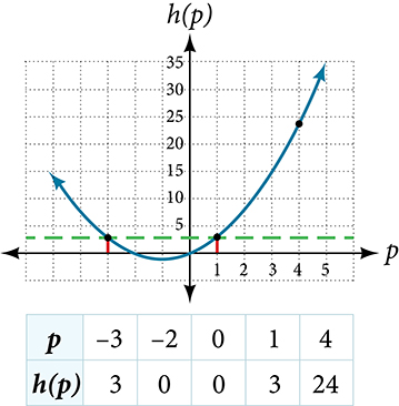
Graph of a parabola with labeled points (-3, 3), (1, 3), and (4, 24).

Figure 3

Try It 1.1.29

Given the function $g(m) = \sqrt{m - 4},$ solve $g(m) = 2.$

Solution (click to reveal)

$m = 8$

Evaluating Functions Expressed in Formulas

Some functions are defined by mathematical rules or procedures expressed in equation form. If it is possible to express the function output with a formula involving the input quantity, then we can define a function in algebraic form. For example, the equation $2n + 6p = 12$ expresses a functional relationship between $n$ and $p.$ We can rewrite it to decide if $p$ is a function of $n.$

How To 1.1.30

Given a function in equation form, write its algebraic formula.

Solve the equation to isolate the output variable on one side of the equal sign, with the other side as an expression that involves only the input variable.
Use all the usual algebraic methods for solving equations, such as adding or subtracting the same quantity to or from both sides, or multiplying or dividing both sides of the equation by the same quantity.

Example 1.1.31 — Finding the Algebraic Form of a Function

Express the relationship $2n + 6p = 12$ as a function $p = f(n),$ if possible.

Solution (click to reveal)

To express the relationship in this form, we need to be able to write the relationship where $p$ is a function of $n,$ which means writing it as $p = \lbrack\text{expression}\mspace{9mu}\text{involving}\mspace{9mu} n\rbrack.$

\[\begin{array}{ll} {2n + 6p = 12} & \\ {\mspace{9mu}\mspace{9mu}\mspace{9mu}\mspace{9mu}\mspace{9mu}\mspace{9mu}\mspace{9mu}\mspace{9mu}\mspace{9mu}\mspace{9mu}\mspace{9mu}\mspace{9mu}\mspace{9mu} 6p = 12 - 2n} & {\begin{array}{lll} & & \end{array}\text{Subtract~}2n\mspace{9mu}\text{from~both~sides}.} \\ {\mspace{9mu}\mspace{9mu}\mspace{9mu}\mspace{9mu}\mspace{9mu}\mspace{9mu}\mspace{9mu}\mspace{9mu}\mspace{9mu}\mspace{9mu}\mspace{9mu}\mspace{9mu}\mspace{9mu}\mspace{9mu}\mspace{9mu}\mspace{9mu} p = \frac{12 - 2n}{6}} & {\begin{array}{lll} & & \end{array}\text{Divide~both~sides~by~6~and~simplify}.} \\ {\mspace{9mu}\mspace{9mu}\mspace{9mu}\mspace{9mu}\mspace{9mu}\mspace{9mu}\mspace{9mu}\mspace{9mu}\mspace{9mu}\mspace{9mu}\mspace{9mu}\mspace{9mu}\mspace{9mu}\mspace{9mu}\mspace{9mu}\mspace{9mu} p = \frac{12}{6} - \frac{2n}{6}} & \\ {\mspace{9mu}\mspace{9mu}\mspace{9mu}\mspace{9mu}\mspace{9mu}\mspace{9mu}\mspace{9mu}\mspace{9mu}\mspace{9mu}\mspace{9mu}\mspace{9mu}\mspace{9mu}\mspace{9mu}\mspace{9mu}\mspace{9mu}\mspace{9mu} p = 2 - \frac{1}{3}n} & \end{array}\]

Therefore, $p$ as a function of $n$ is written as

\[p = f(n) = 2 - \frac{1}{3}n\]

It is important to note that not every relationship expressed by an equation can also be expressed as a function with a formula.

Example 1.1.32 — Expressing the Equation of a Circle as a Function

Does the equation $x^{2} + y^{2} = 1$ represent a function with $x$ as input and $y$ as output? If so, express the relationship as a function $y = f(x).$

Solution (click to reveal)

First we subtract $x^{2}$ from both sides.

\[y^{2} = 1 - x^{2}\]

We now try to solve for $y$ in this equation.

\[\begin{array}{l} {y = \pm \sqrt{1 - x^{2}}} \\ {\mspace{9mu}\ = + \sqrt{1 - x^{2}}\mspace{9mu}\text{and~} - \sqrt{1 - x^{2}}} \end{array}\]

We get two outputs corresponding to the same input, so this relationship cannot be represented as a single function $y = f(x).$

Try It 1.1.33

If $x - 8y^{3} = 0,$ express $y$ as a function of $x.$

Solution (click to reveal)

$y = f(x) = \frac{\sqrt[3]{x}}{2}$

Q&A 1.1.34

Are there relationships expressed by an equation that do represent a function but which still cannot be represented by an algebraic formula?

Yes, this can happen. For example, given the equation $x = y + 2^{y},$ if we want to express $y$ as a function of $x,$ there is no simple algebraic formula involving only $x$ that equals $y.$ However, each $x$ does determine a unique value for $y,$ and there are mathematical procedures by which $y$ can be found to any desired accuracy. In this case, we say that the equation gives an implicit (implied) rule for $y$ as a function of $x,$ even though the formula cannot be written explicitly.

Evaluating a Function Given in Tabular Form

As we saw above, we can represent functions in tables. Conversely, we can use information in tables to write functions, and we can evaluate functions using the tables. For example, how well do our pets recall the fond memories we share with them? There is an urban legend that a goldfish has a memory of 3 seconds, but this is just a myth. Goldfish can remember up to 3 months, while the beta fish has a memory of up to 5 months. And while a puppy’s memory span is no longer than 30 seconds, the adult dog can remember for 5 minutes. This is meager compared to a cat, whose memory span lasts for 16 hours.

The function that relates the type of pet to the duration of its memory span is more easily visualized with the use of a table. See Table 1.1.35.

Pet	Memory span in hours
Puppy	0.008
Adult dog	0.083
Cat	16
Goldfish	2160
Beta fish	3600

Table 1.1.35:

At times, evaluating a function in table form may be more useful than using equations.Here let us call the function $P.$ The domain of the function is the type of pet and the range is a real number representing the number of hours the pet’s memory span lasts. We can evaluate the function $P$ at the input value of “goldfish.” We would write $P(\text{goldfish}) = 2160.$ Notice that, to evaluate the function in table form, we identify the input value and the corresponding output value from the pertinent row of the table. The tabular form for function $P$ seems ideally suited to this function, more so than writing it in paragraph or function form.

How To 1.1.36

Given a function represented by a table, identify specific output and input values.

Find the given input in the row (or column) of input values.
Identify the corresponding output value paired with that input value.
Find the given output values in the row (or column) of output values, noting every time that output value appears.
Identify the input value(s) corresponding to the given output value.

Example 1.1.37 — Evaluating and Solving a Tabular Function

Using Table 1.1.38,
ⓐ Evaluate $g(3).$
ⓑ Solve $g(n) = 6.$

$n$	1	2	3	4	5
$g(n)$	8	6	7	6	8

Table 1.1.38:

Solution (click to reveal)

ⓐ Evaluating $g(3)$ means determining the output value of the function $g$ for the input value of $n = 3.$ The table output value corresponding to $n = 3$ is 7, so $g(3) = 7.$
ⓑ Solving $g(n) = 6$ means identifying the input values, $n,$ that produce an output value of 6. The table below shows two solutions: $2$ and $4.$

$n$	1	2	3	4	5
$g(n)$	8	6	7	6	8

When we input 2 into the function $g,$ our output is 6. When we input 4 into the function $g,$ our output is also 6.

Try It 1.1.39

Using the table from Evaluating and Solving a Tabular Function above, evaluate $g(1).$

Solution (click to reveal)

$g(1) = 8$

Finding Function Values from a Graph

Evaluating a function using a graph also requires finding the corresponding output value for a given input value, only in this case, we find the output value by looking at the graph. Solving a function equation using a graph requires finding all instances of the given output value on the graph and observing the corresponding input value(s).

Example 1.1.40 — Reading Function Values from a Graph

Given the graph in Figure 1.1.41,

ⓐ Evaluate $f(2).$
ⓑ Solve $f(x) = 4.$

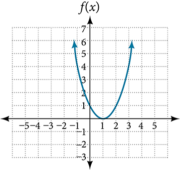
Figure 1.1.41:

Solution (click to reveal)

ⓐ To evaluate $f(2),$ locate the point on the curve where $x = 2,$ then read the $y$-coordinate of that point. The point has coordinates $(2,1),$ so $f(2) = 1.$ See Figure 5.

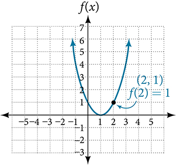
Figure 5

ⓑ To solve $f(x) = 4,$ we find the output value $4$ on the vertical axis. Moving horizontally along the line $y = 4,$ we locate two points of the curve with output value $4:$ $(-1,4)$ and $(3,4).$ These points represent the two solutions to $f(x) = 4:$ $-1$ or $3.$ This means $f(-1) = 4$ and $f(3) = 4,$ or when the input is $-1$ or $\text{3,}$ the output is $\text{4}\text{.}$ See Figure 6.

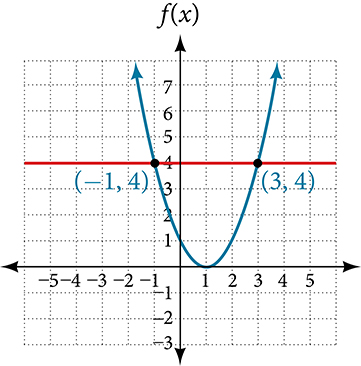
Figure 6

Try It 1.1.42

Using Figure 1.1.41, solve $f(x) = 1.$

Solution (click to reveal)

$x = 0$ or $x = 2$

1.1.3 Determining Whether a Function is One-to-One

Some functions have a given output value that corresponds to two or more input values. For example, in the stock chart shown in the figure at the beginning of this chapter, the stock price was $1000 on five different dates, meaning that there were five different input values that all resulted in the same output value of $1000.

However, some functions have only one input value for each output value, as well as having only one output for each input. We call these functions one-to-one functions. As an example, consider a school that uses only letter grades and decimal equivalents, as listed in Table 1.1.43.

Letter grade	Grade point average
A	4.0
B	3.0
C	2.0
D	1.0

Table 1.1.43:

This grading system represents a one-to-one function, because each letter input yields one particular grade point average output and each grade point average corresponds to one input letter.

To visualize this concept, let’s look again at the two simple functions sketched in Figure 1.1.1(a) and Figure 1.1.1(b). The function in part (a) shows a relationship that is not a one-to-one function because inputs $q$ and $r$ both give output $n.$ The function in part (b) shows a relationship that is a one-to-one function because each input is associated with a single output.

Definition 1.1.44 — One-to-One Function

A one-to-one function is a function in which each output value corresponds to exactly one input value.

Example 1.1.45 — Determining Whether a Relationship Is a One-to-One Function

Is the area of a circle a function of its radius? If yes, is the function one-to-one?

Solution (click to reveal)

A circle of radius $r$ has a unique area measure given by $A = \pi r^{2},$ so for any input, $r,$ there is only one output, $A.$ The area is a function of radius $r.$

If the function is one-to-one, the output value, the area, must correspond to a unique input value, the radius. Any area measure $A$ is given by the formula $A = \pi r^{2}.$ Because areas and radii are positive numbers, there is exactly one solution: $\sqrt{\frac{A}{\pi}}.$ So the area of a circle is a one-to-one function of the circle’s radius.

Try It 1.1.46

ⓐ Is a balance a function of the bank account number?

ⓑ Is a bank account number a function of the balance?

Solution (click to reveal)

ⓐ yes, because each bank account has a single balance at any given time;

ⓑ no, because several bank account numbers may have the same balance;

Try It 1.1.47

Evaluate the following:
ⓐ If each percent grade earned in a course translates to one letter grade, is the letter grade a function of the percent grade?
ⓑ If so, is the function one-to-one?

Solution (click to reveal)

ⓐ Yes, letter grade is a function of percent grade;

ⓑ No, it is not one-to-one. There are 100 different percent numbers we could get but only about five possible letter grades, so there cannot be only one percent number that corresponds to each letter grade.

1.1.4 Using the Vertical Line Test

As we have seen in some examples above, we can represent a function using a graph. Graphs display a great many input-output pairs in a small space. The visual information they provide often makes relationships easier to understand. By convention, graphs are typically constructed with the input values along the horizontal axis and the output values along the vertical axis.

The most common graphs name the input value $x$ and the output value $y,$ and we say $y$ is a function of $x,$ or $y = f(x)$ when the function is named $f.$ The graph of the function is the set of all points $(x,y)$ in the plane that satisfies the equation $y = f(x).$ If the function is defined for only a few input values, then the graph of the function is only a few points, where the $x$-coordinate of each point is an input value and the $y$-coordinate of each point is the corresponding output value. For example, the black dots on the graph in Figure 1.1.48 tell us that $f(0) = 2$ and $f(6) = 1.$ However, the set of all points $(x,y)$ satisfying $y = f(x)$ is a curve. The curve shown includes $(0,2)$ and $(6,1)$ because the curve passes through those points.

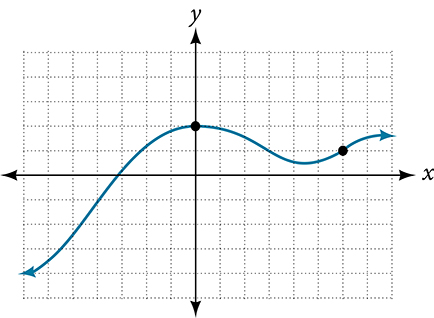
Graph of a smooth curve on a Cartesian coordinate plane. The curve rises from the lower left, passes through the highlighted point (0, 2), levels off briefly, then dips slightly before rising again through the highlighted point (6, 1) and continuing to the right.

Figure 1.1.48:

The vertical line test can be used to determine whether a graph represents a function. If we can draw any vertical line that intersects a graph more than once, then the graph does not define a function because a function has only one output value for each input value. See Figure 1.1.49.

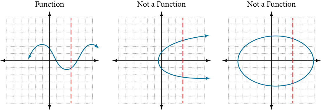
Three graphs visually showing what is and is not a function.

Figure 1.1.49:

How To 1.1.50

Given a graph, use the vertical line test to determine if the graph represents a function.

Inspect the graph to see if any vertical line drawn would intersect the curve more than once.
If there is any such line, determine that the graph does not represent a function.

Example 1.1.51 — Applying the Vertical Line Test

Which of the graphs in Figure 1.1.52 represent(s) a function $y = f(x)?$

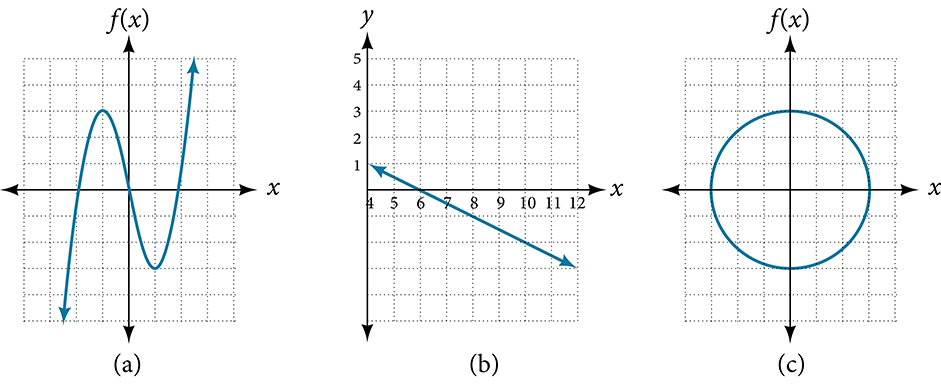
Figure 1.1.52:

Solution (click to reveal)

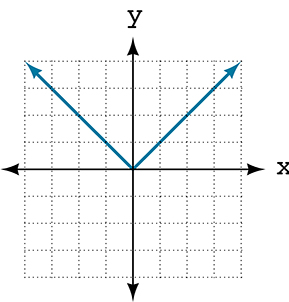
If any vertical line intersects a graph more than once, the relation represented by the graph is not a function. Notice that any vertical line would pass through only one point of the two graphs shown in parts (a) and (b) of Figure 1.1.52. From this we can conclude that these two graphs represent functions. The third graph does not represent a function because, at most $x$-values, a vertical line would intersect the graph at more than one point, as shown in Figure 1.1.54.

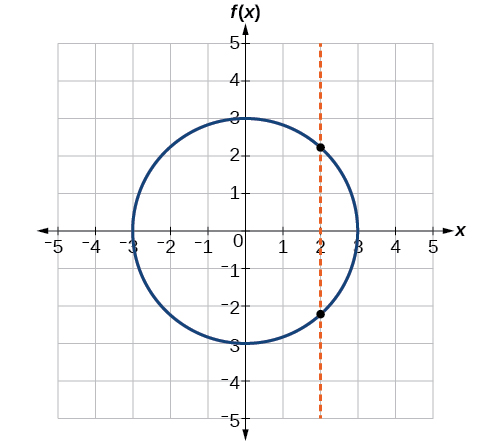
A circle with radius 3 centered at the origin is shown. A vertical dashed line at x=2 intersects the circle at two points, demonstrating that the circle is not a function.

Figure 10

Try It 1.1.53

Does the graph in Figure 1.1.54 represent a function?

Figure 1.1.54:

Solution (click to reveal)

yes

1.1.5 Using the Horizontal Line Test

Once we have determined that a graph defines a function, an easy way to determine if it is a one-to-one function is to use the horizontal line test. Draw horizontal lines through the graph. If any horizontal line intersects the graph more than once, then the graph does not represent a one-to-one function.

How To 1.1.55

Given a graph of a function, use the horizontal line test to determine if the graph represents a one-to-one function.

Inspect the graph to see if any horizontal line drawn would intersect the curve more than once.
If there is any such line, determine that the function is not one-to-one.

Example 1.1.56 — Applying the Horizontal Line Test

Consider the functions shown in Figure 1.1.52(a) and Figure 1.1.52(b). Are either of the functions one-to-one?

Solution (click to reveal)

The function in Figure 1.1.52(a) is not one-to-one. The horizontal line shown in Figure 12 intersects the graph of the function at two points (and we can even find horizontal lines that intersect it at three points.)

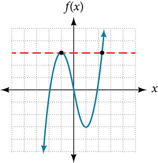
A blue curve representing a function f(x) intersects a horizontal red dashed line at two black-dotted points on a grid, illustrating solutions to f(x)=c for a constant c.

Figure 12

The function in Figure 1.1.52(b) is one-to-one. Any horizontal line will intersect a diagonal line at most once.

Try It 1.1.57

Is the graph shown in Figure 1.1.52(c) one-to-one?

Solution (click to reveal)

No, because it does not pass the horizontal line test.

1.1.6 Identifying Basic Toolkit Functions

In this text, we will be exploring functions—the shapes of their graphs, their unique characteristics, their algebraic formulas, and how to solve problems with them. When learning to read, we start with the alphabet. When learning to do arithmetic, we start with numbers. When working with functions, it is similarly helpful to have a base set of building-block elements. We call these our “toolkit functions,” which form a set of basic named functions for which we know the graph, formula, and special properties. Some of these functions are programmed to individual buttons on many calculators. For these definitions we will use $x$ as the input variable and $y = f(x)$ as the output variable.

We will see these toolkit functions, combinations of toolkit functions, their graphs, and their transformations frequently throughout this book. It will be very helpful if we can recognize these toolkit functions and their features quickly by name, formula, graph, and basic table properties. The graphs and sample table values are included with each function shown in Table 1.1.58.

Toolkit Functions
Name	Function	Graph
Constant	$f(x) = c,$ where $c$ is a constant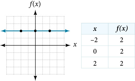
Identity	$f(x) = x$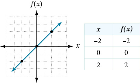
Absolute value	$f(x) = \|x\|$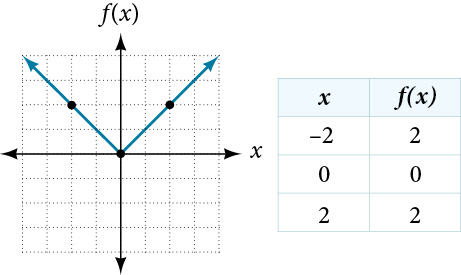
Quadratic	$f(x) = x^{2}$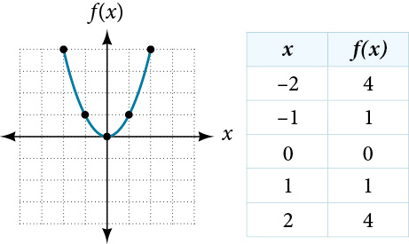
Cubic	$f(x) = x^{3}$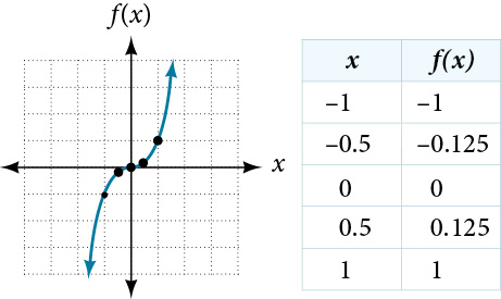
Reciprocal	$f(x) = \frac{1}{x}$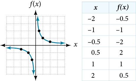
Reciprocal squared	$f(x) = \frac{1}{x^{2}}$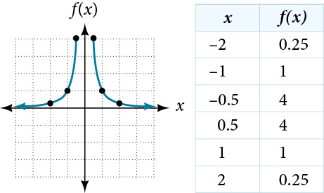
Square root	$f(x) = \sqrt{x}$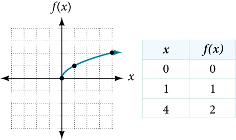
Cube root	$f(x) = \sqrt[3]{x}$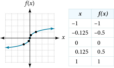

Table 1.1.58:

\(n\)	1	2	3	4	5
\(Q\)	8	6	7	6	8

\(n\)	1	2	3	4	5
\(g(n)\)	8	6	7	6	8

\(n\)	1	2	3	4	5
\(g(n)\)	8	6	7	6	8