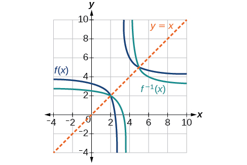
1.7 Inverse Functions
A reversible heat pump is a climate-control system that is an air conditioner and a heater in a single device. Operated in one direction, it pumps heat out of a house to provide cooling. Operating in reverse, it pumps heat into the building from the outside, even in cool weather, to provide heating. As a heater, a heat pump is several times more efficient than conventional electrical resistance heating.
If some physical machines can run in two directions, we might ask whether some of the function “machines” we have been studying can also run backwards. Figure 1.7.1 provides a visual representation of this question. In this section, we will consider the reverse nature of functions.
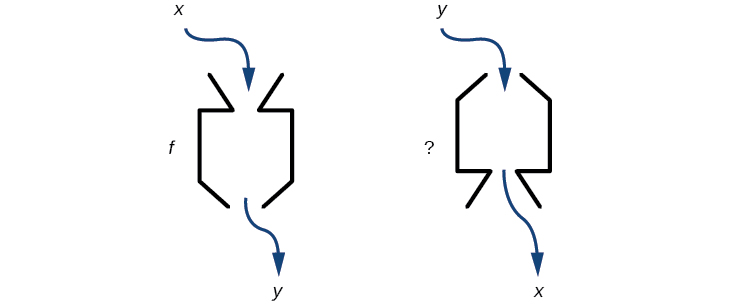
Figure 1.7.1: Can a function “machine” operate in reverse?
1.7.1 Verifying That Two Functions Are Inverse Functions
Betty is traveling to Milan for a fashion show and wants to know what the temperature will be. She is not familiar with the Celsius scale. To get an idea of how temperature measurements are related, Betty wants to convert 75 degrees Fahrenheit to degrees Celsius using the formula
\[C = \frac{5}{9}(F - 32)\]
and substitutes 75 for \(F\) to calculate
\[\frac{5}{9}(75 - 32) \approx 24\text{°C}\]
Knowing that a comfortable 75 degrees Fahrenheit is about 24 degrees Celsius, Betty gets the week’s weather forecast from Figure 1.7.2 for Milan, and wants to convert all of the temperatures to degrees Fahrenheit.
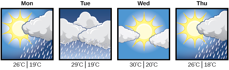
Figure 1.7.2:
At first, Betty considers using the formula she has already found to complete the conversions. After all, she knows her algebra, and can easily solve the equation for \(F\) after substituting a value for \(C.\) For example, to convert 26 degrees Celsius, she could write
\[\begin{array}{rcl} 26 & = & {\frac{5}{9}(F - 32)} \\ {26 \cdot \frac{9}{5}} & = & {F - 32} \\ F & = & {26 \cdot \frac{9}{5} + 32 \approx 79} \end{array}\]
After considering this option for a moment, however, she realizes that solving the equation for each of the temperatures will be awfully tedious. She realizes that since evaluation is easier than solving, it would be much more convenient to have a different formula, one that takes the Celsius temperature and outputs the Fahrenheit temperature.
The formula for which Betty is searching corresponds to the idea of an inverse function, which is a function for which the input of the original function becomes the output of the inverse function and the output of the original function becomes the input of the inverse function.
Given a function \(f(x),\) we represent its inverse as \(f^{- 1}(x),\) read as \(``f\) inverse of \(x.\text{”}\) The raised \(-1\) is part of the notation. It is not an exponent; it does not imply a power of \(-1\) . In other words, \(f^{- 1}(x)\) does not mean \(\frac{1}{f(x)}\) because \(\frac{1}{f(x)}\) is the reciprocal of \(f\) and not the inverse.
The “exponent-like” notation comes from an analogy between function composition and multiplication: just as \(a^{- 1}a = 1\) (1 is the identity element for multiplication) for any nonzero number \(a,\) so \(f^{- 1} \circ f\) equals the identity function, that is,
\[\left( {f^{- 1} \circ f} \right)(x) = f^{- 1}\left( {f(x)} \right) = f^{- 1}(y) = x\]
This holds for all \(x\) in the domain of \(f.\) Informally, this means that inverse functions “undo” each other. However, just as zero does not have a reciprocal, some functions do not have inverses.
Given a function \(f(x),\) we can verify whether some other function \(g(x)\) is the inverse of \(f(x)\) by checking if both \(g(f(x)) = x\) and \(f(g(x)) = x\) are true.
For example, \(y = 4x\) and \(y = \frac{1}{4}x\) are inverse functions.
\[\left( {f^{- 1} \circ f} \right)(x) = f^{- 1}\left( {4x} \right) = \frac{1}{4}\left( {4x} \right) = x\]
and
\[\left( {f^{} \circ f^{- 1}} \right)(x) = f\left( {\frac{1}{4}x} \right) = 4\left( {\frac{1}{4}x} \right) = x\]
A few coordinate pairs from the graph of the function \(y = 4x\) are (−2, −8), (0, 0), and (2, 8). A few coordinate pairs from the graph of the function \(y = \frac{1}{4}x\) are (−8, −2), (0, 0), and (8, 2). If we interchange the input and output of each coordinate pair of a function, the interchanged coordinate pairs would appear on the graph of the inverse function.
1.7.2 Finding Domain and Range of Inverse Functions
The outputs of the function \(f\) are the inputs to \(f^{- 1},\) so the range of \(f\) is also the domain of \(f^{- 1}.\) Likewise, because the inputs to \(f\) are the outputs of \(f^{- 1},\) the domain of \(f\) is the range of \(f^{- 1}.\) We can visualize the situation as in Figure 1.7.12.
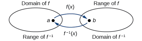
Figure 1.7.12: Domain and range of a function and its inverse
When a function has no inverse function, it is possible to create a new function where that new function on a limited domain does have an inverse function. For example, the inverse of \(f(x) = \sqrt{x}\) is \(f^{- 1}(x) = x^{2},\) because a square “undoes” a square root; but the square is only the inverse of the square root on the domain \(\left\lbrack {0,\infty} \right),\) since that is the range of \(f(x) = \sqrt{x}.\)
We can look at this problem from the other side, starting with the square (toolkit quadratic) function \(f(x) = x^{2}.\) If we want to construct an inverse to this function, we run into a problem, because for every given output of the quadratic function, there are two corresponding inputs (except when the input is 0). For example, the output 9 from the quadratic function corresponds to the inputs 3 and –3. But an output from a function is an input to its inverse; if this inverse input corresponds to more than one inverse output (input of the original function), then the “inverse” is not a function at all! To put it differently, the quadratic function is not a one-to-one function; it fails the horizontal line test, so it does not have an inverse function. In order for a function to have an inverse, it must be a one-to-one function.
In many cases, if a function is not one-to-one, we can still restrict the function to a part of its domain on which it is one-to-one. For example, we can make a restricted version of the square function \(f(x) = x^{2}\) with its domain limited to \(\left\lbrack {0,\infty} \right),\) which is a one-to-one function (it passes the horizontal line test) and which has an inverse (the square-root function).
If \(f(x) = \left( {x - 1} \right)^{2}\) on \(\left\lbrack {1,\infty} \right),\) then the inverse function is \(f^{- 1}(x) = \sqrt{x} + 1.\)
- The domain of \(f\) = range of \(f^{- 1}\) = \(\left\lbrack {1,\infty} \right).\)
- The domain of \(f^{- 1}\) = range of \(f\) = \(\left\lbrack {0,\infty} \right).\)
Identify which of the toolkit functions besides the quadratic function are not one-to-one, and find a restricted domain on which each function is one-to-one, if any. The toolkit functions are reviewed in Table 1.7.17. We restrict the domain in such a fashion that the function assumes all \(y\)-values exactly once.
| Constant | Identity | Quadratic | Cubic | Reciprocal |
|---|---|---|---|---|
| \(f(x) = c\) | \(f(x) = x\) | \(f(x) = x^{2}\) | \(f(x) = x^{3}\) | \(f(x) = \frac{1}{x}\) |
| Reciprocal squared | Cube root | Square root | Absolute value | |
| \(f(x) = \frac{1}{x^{2}}\) | \(f(x) = \sqrt[3]{x}\) | \(f(x) = \sqrt{x}\) | \(f(x) = |x|\) |
Table 1.7.17:
Solution (click to reveal)
The constant function is not one-to-one, and there is no domain (except a single point) on which it could be one-to-one, so the constant function has no inverse.
The absolute value function can be restricted to the domain \(\left\lbrack {0,\infty} \right),\) where it is equal to the identity function.
The reciprocal-squared function can be restricted to the domain \(\left( {0,\infty} \right).\)
We can see that these functions (if unrestricted) are not one-to-one by looking at their graphs, shown in Figure 1.7.18. They both would fail the horizontal line test. However, if a function is restricted to a certain domain so that it passes the horizontal line test, then in that restricted domain, it can have an inverse.
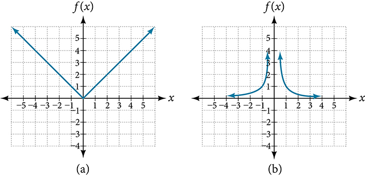
Figure 1.7.18: (a) Absolute value (b) Reciprocal square
1.7.3 Finding and Evaluating Inverse Functions
Once we have a one-to-one function, we can evaluate its inverse at specific inverse function inputs or construct a complete representation of the inverse function in many cases.
Inverting Tabular Functions
Suppose we want to find the inverse of a function represented in table form. Remember that the domain of a function is the range of the inverse and the range of the function is the domain of the inverse. So we need to interchange the domain and range.
Each row (or column) of inputs becomes the row (or column) of outputs for the inverse function. Similarly, each row (or column) of outputs becomes the row (or column) of inputs for the inverse function.
Evaluating the Inverse of a Function, Given a Graph of the Original Function
We saw in Functions and Function Notation that the domain of a function can be read by observing the horizontal extent of its graph. We find the domain of the inverse function by observing the vertical extent of the graph of the original function, because this corresponds to the horizontal extent of the inverse function. Similarly, we find the range of the inverse function by observing the horizontal extent of the graph of the original function, as this is the vertical extent of the inverse function. If we want to evaluate an inverse function, we find its input within its domain, which is all or part of the vertical axis of the original function’s graph.
A function \(g(x)\) is given in Figure 1.7.26. Find \(g(3)\) and \(g^{- 1}(3).\)
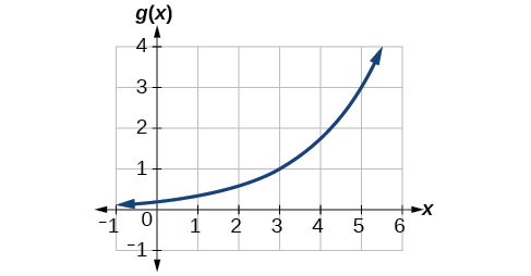
Figure 1.7.26:
Solution (click to reveal)
To evaluate \(g(3),\) we find 3 on the \(x\)-axis and find the corresponding output value on the \(y\)-axis. The point \(\left( {3,1} \right)\) tells us that \(g(3) = 1.\)
To evaluate \(g^{- 1}(3),\) recall that by definition \(g^{- 1}(3)\) means the value of \(x\) for which \(g(x) = 3.\) By looking for the output value 3 on the vertical axis, we find the point \(\left( {5,3} \right)\) on the graph, which means \(g(5) = 3,\) so by definition, \(g^{- 1}(3) = 5.\) See Table 1.7.32.
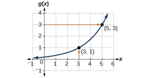
Figure 6
Finding Inverses of Functions Represented by Formulas
Sometimes we will need to know an inverse function for all elements of its domain, not just a few. If the original function is given as a formula—for example, \(y\) as a function of \(x\text{—}\) we can often find the inverse function by solving to obtain \(x\) as a function of \(y.\)
1.7.4 Finding Inverse Functions and Their Graphs
Now that we can find the inverse of a function, we will explore the graphs of functions and their inverses. Let us return to the quadratic function \(f(x) = x^{2}\) restricted to the domain \(\lbrack 0,\infty)\text{,}\) on which this function is one-to-one, and graph it as in Figure 1.7.35.
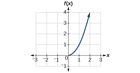
Figure 1.7.35: Quadratic function with domain restricted to [0, ∞).
Restricting the domain to \(\lbrack 0,\infty)\) makes the function one-to-one (it will obviously pass the horizontal line test), so it has an inverse on this restricted domain.
We already know that the inverse of the toolkit quadratic function is the square root function, that is, \(f^{- 1}(x) = \sqrt{x}.\) What happens if we graph both \(f\) and \(f^{- 1}\) on the same set of axes, using the \(x\text{-}\) axis for the input to both \(f\mspace{9mu}\text{and~~}f^{- 1}?\)
We notice a distinct relationship: The graph of \(f^{- 1}(x)\) is the graph of \(f(x)\) reflected about the diagonal line \(y = x,\) which we will call the identity line, shown in Figure 1.7.36.
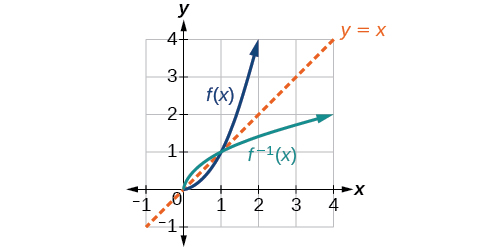
Figure 1.7.36: Square and square-root functions on the non-negative domain
This relationship will be observed for all one-to-one functions, because it is a result of the function and its inverse swapping inputs and outputs. This is equivalent to interchanging the roles of the vertical and horizontal axes.
Given the graph of \(f(x)\) in Figure 1.7.38, sketch a graph of \(f^{- 1}(x).\)
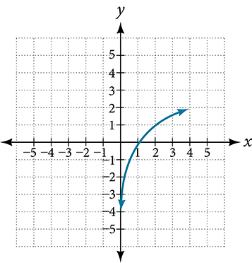
Figure 1.7.38:
Solution (click to reveal)
This is a one-to-one function, so we will be able to sketch an inverse. Note that the graph shown has an apparent domain of \(\left( {0,\infty} \right)\) and range of \(\left( {- \infty,\infty} \right),\) so the inverse will have a domain of \(\left( {- \infty,\infty} \right)\) and range of \(\left( {0,\infty} \right).\)
If we reflect this graph over the line \(y = x,\) the point \(\left( {1,0} \right)\) reflects to \(\left( {0,1} \right)\) and the point \(\left( {4,2} \right)\) reflects to \(\left( {2,4} \right).\) Sketching the inverse on the same axes as the original graph gives Figure 10.
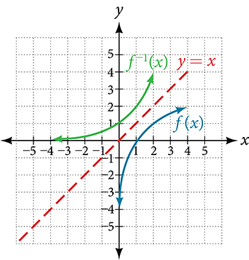
Figure 10 The function and its inverse, showing reflection about the identity line
Draw graphs of the functions \(f\) and \(f^{- 1}\) from Example 8.
Solution (click to reveal)