1.3 Rates of Change and Behavior of Graphs
Gasoline costs have experienced some wild fluctuations over the last several decades. The table below lists the average cost, in dollars, of a gallon of gasoline for the years 2005–2012. The cost of gasoline can be considered as a function of year.
| \(y\) | 2005 | 2006 | 2007 | 2008 | 2009 | 2010 | 2011 | 2012 |
|---|---|---|---|---|---|---|---|---|
| \(C(y)\) | 2.31 | 2.62 | 2.84 | 3.30 | 2.41 | 2.84 | 3.58 | 3.68 |
Table 1.3.1: Average cost in dollars of a gallon of gasoline, 2005–2012.
If we were interested only in how the gasoline prices changed between 2005 and 2012, we could compute that the cost per gallon had increased from $2.31 to $3.68, an increase of $1.37. While this is interesting, it might be more useful to look at how much the price changed per year. In this section, we will investigate changes such as these.
1.3.1 Finding the Average Rate of Change of a Function
The price change per year is a rate of change because it describes how an output quantity changes relative to the change in the input quantity. We can see that the price of gasoline in Table 1.3.1 did not change by the same amount each year, so the rate of change was not constant. If we use only the beginning and ending data, we would be finding the average rate of change over the specified period of time. To find the average rate of change, we divide the change in the output value by the change in the input value.
\[\begin{array}{ccl} {\text{Average~rate~of~change}} & = & \frac{\text{Change~in~output}}{\text{Change~in~input}} \\ & = & \frac{\Delta y}{\Delta x} \\ & = & \frac{y_{2} - y_{1}}{x_{2} - x_{1}} \\ & = & \frac{f\left( x_{2} \right) - f\left( x_{1} \right)}{x_{2} - x_{1}} \end{array}\]
The Greek letter \(\text{Δ}\) (delta) signifies the change in a quantity; we read the ratio as “delta-\(y\) over delta-\(x\)” or “the change in \(y\) divided by the change in \(x.\)” Occasionally we write \(\text{Δ}f\) instead of \(\text{Δ}y,\) which still represents the change in the function’s output value resulting from a change to its input value. It does not mean we are changing the function into some other function.
In our example, the gasoline price increased by $1.37 from 2005 to 2012. Over 7 years, the average rate of change was
\[\frac{\text{Δ}y}{\text{Δ}x} = \frac{\text{\$}1.37}{\text{7~years}} \approx 0.196\mspace{9mu}\text{dollars~per~year}\]
On average, the price of gas increased by about 19.6¢ each year.
Other examples of rates of change include:
- A population of rats increasing by 40 rats per week
- A car traveling 68 miles per hour (distance traveled changes by 68 miles each hour as time passes)
- A car driving 27 miles per gallon (distance traveled changes by 27 miles for each gallon)
- The current through an electrical circuit increasing by 0.125 amperes for every volt of increased voltage
- The amount of money in a college account decreasing by $4,000 per quarter
Given the function \(g(t)\), find the average rate of change on the interval \(\left\lbrack {- 1,2} \right\rbrack.\)
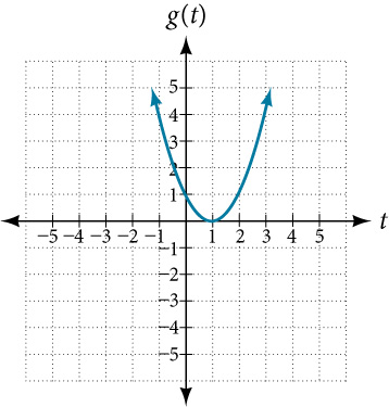
Figure 1.3.1: The graph of \(g(t)\) for Example 1.3.6.
Solution
At \(t = - 1,\) \(g(-1) = 4.\) At \(t = 2,\) the graph shows \(g(2) = 1.\)
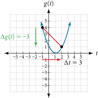
Figure: Secant line through \((-1,\, 4)\) and \((2,\, 1)\) visualizes the average rate of change.
The horizontal change \(\text{Δ}t = 3\) is shown by the red arrow, and the vertical change \(\text{Δ}g(t) = - 3\) is shown by the turquoise arrow. The average rate of change is shown by the slope of the orange line segment. The output changes by –3 while the input changes by 3, giving an average rate of change of
\[\frac{1 - 4}{2 - \left( {- 1} \right)} = \frac{- 3}{3} = -1\]
Analysis. Note that the order we choose is very important. If, for example, we use \(\frac{y_{2} - y_{1}}{x_{1} - x_{2}},\) we will not get the correct answer. Decide which point will be 1 and which point will be 2, and keep the coordinates fixed as \(\left( {x_{1},y_{1}} \right)\) and \(\left( {x_{2},y_{2}} \right).\)
1.3.2 The Difference Quotient
When studying rates of change, we often want to examine what happens near a particular input value \(x\). Instead of using two separate variables \(a\) and \(b\), we use \(x\) for our starting point and \(x + h\) for a nearby point, where \(h\) represents a small horizontal shift.
With this notation, \(b - a\) becomes \((x + h) - x = h\), and the average rate of change formula transforms into the difference quotient.
Let’s break down what this expression means:
- \(f(x)\) is the output of our function at some starting point \(x\).
- \(f(x + h)\) is the output at a nearby point, where \(h\) represents a small horizontal shift.
- The numerator \(f(x + h) - f(x)\) measures how much the output changed.
- Dividing by \(h\) tells us the change in output per unit of input.
Geometrically, the difference quotient gives the slope of the secant line connecting the points \((x, f(x))\) and \((x + h, f(x + h))\) on the graph of \(f\), as shown in Figure 1.3.2.
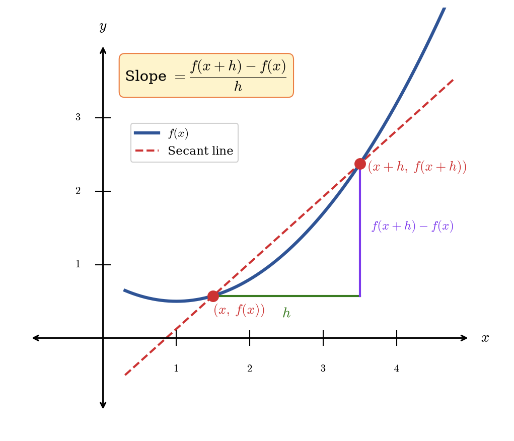
Figure 1.3.2: The difference quotient as the slope of a secant line through \((x, f(x))\) and \((x + h, f(x + h))\).
Why does this matter?
The difference quotient appears throughout science and engineering:
- Physics: Average velocity is the difference quotient of position with respect to time.
- Economics: Marginal cost approximations use difference quotients to estimate how costs change with production levels.
- Biology: Population growth rates are computed as difference quotients of population size over time.
In calculus, you’ll take the limit of the difference quotient as \(h\) approaches zero, which gives the instantaneous rate of change—the derivative. Mastering the algebraic techniques in this section will prepare you for that transition.
1.3.3 Computing Difference Quotients
Computing a difference quotient is a three-step process: find \(f(x + h)\), compute \(f(x + h) - f(x)\), and divide by \(h\) and simplify. The algebra varies depending on the type of function. Let’s work through the main cases.
Compute the difference quotient for \(f(x) = 2x^2 + x - 5\).
Solution
Step 1: Find \(f(x + h)\) by replacing every \(x\) with \((x + h)\):
\[ f(x + h) = 2(x + h)^2 + (x + h) - 5 \]
Expand \((x + h)^2 = x^2 + 2xh + h^2\):
\[ f(x + h) = 2(x^2 + 2xh + h^2) + x + h - 5 = 2x^2 + 4xh + 2h^2 + x + h - 5 \]
Step 2: Compute \(f(x + h) - f(x)\):
\[ f(x + h) - f(x) = (2x^2 + 4xh + 2h^2 + x + h - 5) - (2x^2 + x - 5) = 4xh + 2h^2 + h \]
Step 3: Divide by \(h\):
\[ \frac{f(x + h) - f(x)}{h} = \frac{4xh + 2h^2 + h}{h} = \frac{h(4x + 2h + 1)}{h} = 4x + 2h + 1 \]
Result: The difference quotient is \(4x + 2h + 1\).
The figure below illustrates this example with specific values \(x = 1\) and \(h = 1\), giving a secant line with slope \(4(1) + 2(1) + 1 = 7\).
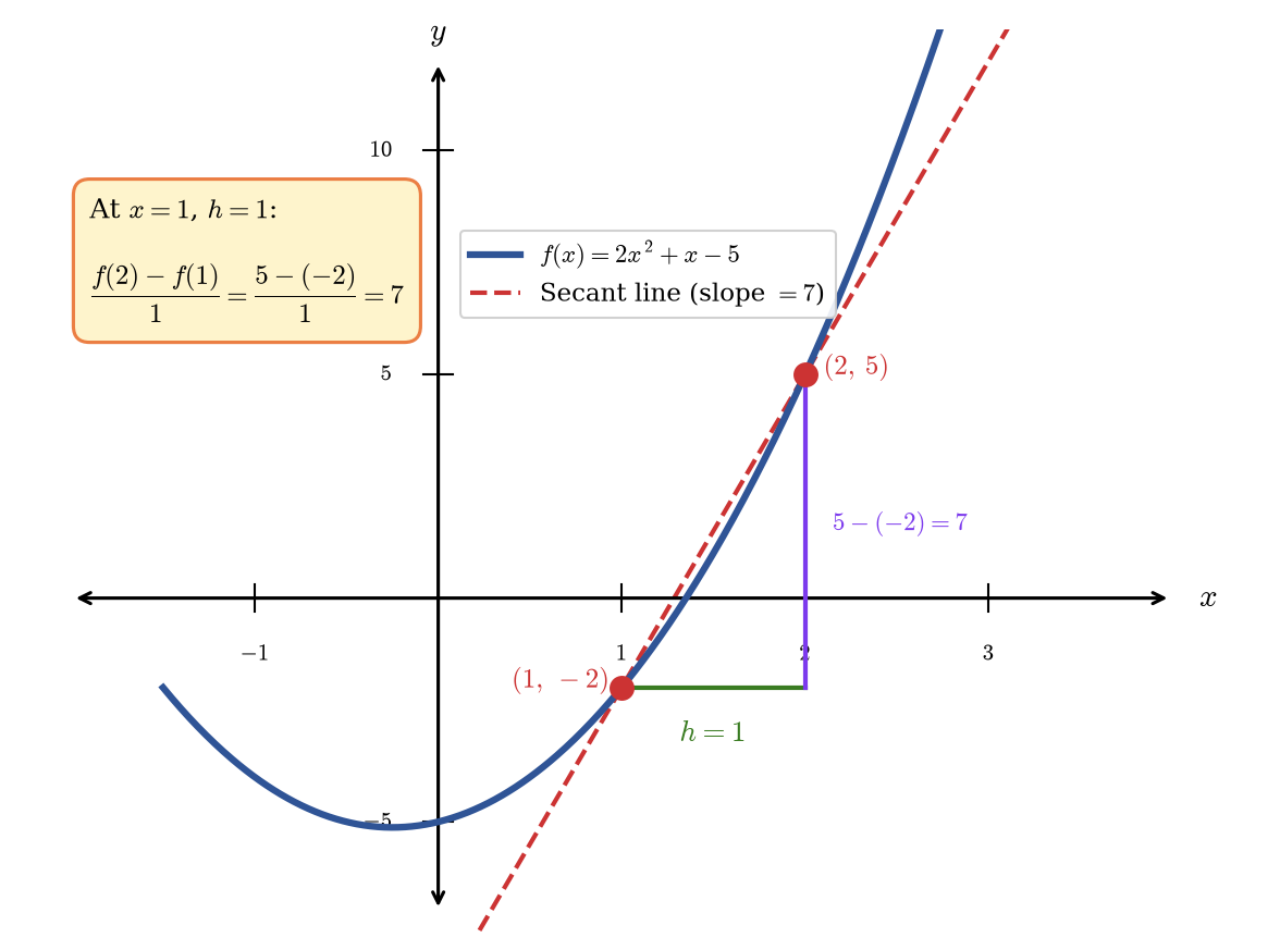
Figure: The secant line for \(f(x) = 2x^2 + x - 5\) with \(x = 1\) and \(h = 1\), showing slope \(= 7\).
Notice that as \(h\) gets smaller, this expression approaches \(4x + 1\)—which, as you’ll learn in calculus, is the derivative of \(f(x) = 2x^2 + x - 5\).
The difference quotient isn’t just an algebraic exercise—it answers a practical question whenever the function represents a measurable quantity. If \(C(x)\) represents cost, then the difference quotient tells us how quickly costs are rising. If \(P(t)\) represents population, it tells us how fast the population is growing.
So far, our difference quotient computations have involved polynomial functions, where the main algebraic challenge is expanding and collecting terms. But the three-step process works for any type of function—the algebra just looks different. When the function involves fractions, finding common denominators becomes the key step.
Functions involving square roots require yet another algebraic technique. When the numerator contains a difference of radicals, we can’t factor or find common denominators—instead, we rationalize by multiplying by the conjugate. This is a technique worth mastering, as it appears frequently in calculus.
Rationalization is especially useful when the function has a physical or scientific meaning, because it lets us simplify the difference quotient into a form where we can substitute specific values and interpret the result.
1.3.4 Using a Graph to Determine Where a Function is Increasing, Decreasing, or Constant
As part of exploring how functions change, we can identify intervals over which the function is changing in specific ways. We say that a function is increasing on an interval if the function values increase as the input values increase within that interval. Similarly, a function is decreasing on an interval if the function values decrease as the input values increase over that interval. The average rate of change of an increasing function is positive, and the average rate of change of a decreasing function is negative. examples of increasing and decreasing intervals on a function.
While some functions are increasing (or decreasing) over their entire domain, many others are not. A value of the input where a function changes from increasing to decreasing (as we go from left to right, that is, as the input variable increases) is the location of a local maximum. The function value at that point is the local maximum. If a function has more than one, we say it has local maxima. Similarly, a value of the input where a function changes from decreasing to increasing as the input variable increases is the location of a local minimum. The function value at that point is the local minimum. The plural form is “local minima.” Together, local maxima and minima are called local extrema, or local extreme values, of the function. (The singular form is “extremum.”) Often, the term local is replaced by the term relative. In this text, we will use the term local.
The figure below shows examples of increasing and decreasing intervals on a function.
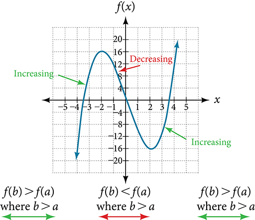
Figure 1.3.3: Examples of increasing and decreasing intervals on a function.
Clearly, a function is neither increasing nor decreasing on an interval where it is constant. A function is also neither increasing nor decreasing at extrema. Note that we have to speak of local extrema, because any given local extremum as defined here is not necessarily the highest maximum or lowest minimum in the function’s entire domain.
For the function whose graph is shown in Figure 1.3.4, the local maximum is 16, and it occurs at \(x = -2.\) The local minimum is \(-16\) and it occurs at \(x = 2.\)
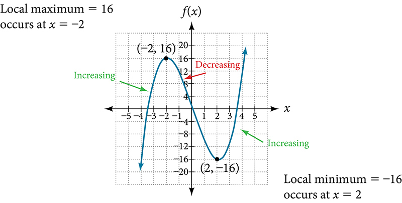
Figure 1.3.4: \(f(x) = x^{3} - 12x\) is increasing on \((-\infty,\, -2) \cup (2,\, \infty)\) and decreasing on \((-2,\, 2)\).
To locate the local maxima and minima from a graph, we need to observe the graph to determine where the graph attains its highest and lowest points, respectively, within an open interval. Like the summit of a roller coaster, the graph of a function is higher at a local maximum than at nearby points on both sides. The graph will also be lower at a local minimum than at neighboring points. The figure below illustrates these ideas for a local maximum.
These observations lead us to a formal definition of local extrema.
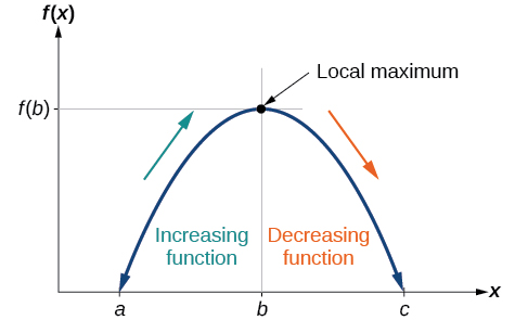
Figure 1.3.5: A local maximum: the output is larger than at any nearby input.
Given the function \(p(t)\) in the figure below, identify the intervals on which the function appears to be increasing.
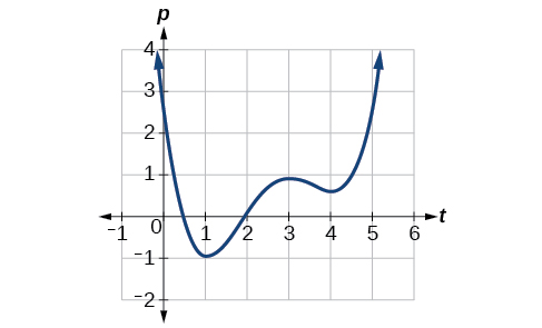
Figure 1.3.6: The graph of \(p(t)\) for Example 1.3.28.
Solution
We see that the function is not constant on any interval. The function is increasing where it slants upward as we move to the right and decreasing where it slants downward as we move to the right. The function appears to be increasing from \(t = 1\) to \(t = 3\) and from \(t = 4\) on.
In interval notation, we would say the function appears to be increasing on the interval (1,3) and the interval \((4,\infty).\)
Analysis. Notice in this example that we used open intervals (intervals that do not include the endpoints), because the function is neither increasing nor decreasing at \(t = 1\) , \(t = 3\) , and \(t = 4\) . These points are the local extrema (two minima and a maximum).
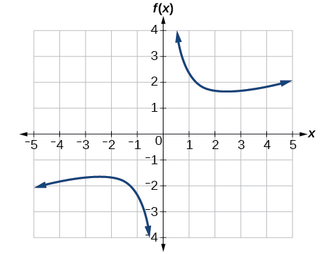
Figure 1.3.7: The graph for Example 1.3.30.
Graph the function \(f(x) = \frac{2}{x} + \frac{x}{3}.\) Then use the graph to estimate the local extrema of the function and to determine the intervals on which the function is increasing.
Solution
Using technology, we find that the graph of the function looks like the graph above. It appears there is a low point, or local minimum, between \(x = 2\) and \(x = 3,\) and a mirror-image high point, or local maximum, somewhere between \(x = -3\) and \(x = -2.\)
Analysis. Most graphing calculators and graphing utilities can estimate the location of maxima and minima. The figure below provides screen images from two different technologies, showing the estimate for the local maximum and minimum.
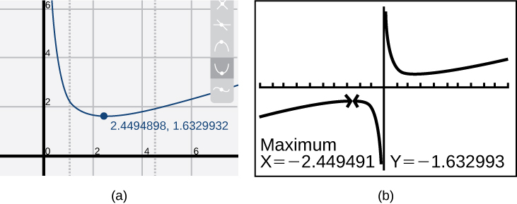
Figure: Calculator estimates of the local maximum and minimum.
Based on these estimates, the function is increasing on the interval \(( - \infty\ \text{,} - \text{2}\text{.449)}\) and \((2.449\ \text{,}\infty).\) Notice that, while we expect the extrema to be symmetric, the two different technologies agree only up to four decimals due to the differing approximation algorithms used by each. (The exact location of the extrema is at \(\pm \sqrt{6},\) but determining this requires calculus.)
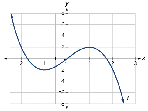
Figure 1.3.8: The graph of \(f\) for Example 1.3.33.
For the function \(f\) whose graph is shown in Figure 1.3.8, find all local maxima and minima.
Solution
Observe the graph of \(f.\) The graph attains a local maximum at \(x = 1\) because it is the highest point in an open interval around \(x = 1.\) The local maximum is the \(y\) -coordinate at \(x = 1,\) which is \(2.\)
The graph attains a local minimum at \(x = -1\) because it is the lowest point in an open interval around \(x = -1.\) The local minimum is the \(y\)-coordinate at \(x = -1,\) which is \(-2.\)
1.3.5 Analyzing the Toolkit Functions for Increasing or Decreasing Intervals
We will now return to our toolkit functions and summarize their graphical behavior. The table below records each function’s formula, domain, and the intervals on which it is increasing, decreasing, or constant.
| Function | Formula | Domain | Behavior | Graph |
|---|---|---|---|---|
| Constant | \(f(x) = c\) | \((-\infty, \infty)\) | Constant on \((-\infty, \infty)\) | 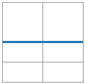 |
| Identity | \(f(x) = x\) | \((-\infty, \infty)\) | Increasing on \((-\infty, \infty)\) | 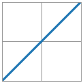 |
| Quadratic | \(f(x) = x^{2}\) | \((-\infty, \infty)\) | Decreasing on \((-\infty, 0)\); increasing on \((0, \infty)\); minimum at \(x = 0\) | 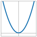 |
| Cubic | \(f(x) = x^{3}\) | \((-\infty, \infty)\) | Increasing on \((-\infty, \infty)\) | 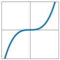 |
| Reciprocal | \(f(x) = \dfrac{1}{x}\) | \((-\infty,0)\cup(0,\infty)\) | Decreasing on \((-\infty, 0)\) and on \((0, \infty)\) | 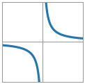 |
| Reciprocal sq. | \(f(x) = \dfrac{1}{x^{2}}\) | \((-\infty,0)\cup(0,\infty)\) | Increasing on \((-\infty, 0)\); decreasing on \((0, \infty)\) | 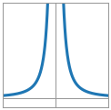 |
| Cube root | \(f(x) = \sqrt[3]{x}\) | \((-\infty, \infty)\) | Increasing on \((-\infty, \infty)\) | 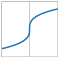 |
| Square root | \(f(x) = \sqrt{x}\) | \([0, \infty)\) | Increasing on \([0, \infty)\); minimum at \(x = 0\) | 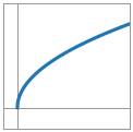 |
| Absolute value | \(f(x) = \lvert x \rvert\) | \((-\infty, \infty)\) | Decreasing on \((-\infty, 0)\); increasing on \((0, \infty)\); minimum at \(x = 0\) | 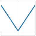 |
Table 1.3.35: Toolkit functions and their increasing/decreasing/constant intervals.
1.3.6 Use A Graph to Locate the Absolute Maximum and Absolute Minimum
There is a difference between locating the highest and lowest points on a graph in a region around an open interval (locally) and locating the highest and lowest points on the graph for the entire domain. The \(y\ \text{-}\) coordinates (output) at the highest and lowest points are called the absolute maximum and absolute minimum, respectively.
To locate absolute maxima and minima from a graph, we need to observe the graph to determine where the graph attains it highest and lowest points on the domain of the function. Not every function has an absolute maximum or minimum value. The toolkit function \(f(x) = x^{3}\) is one such function.
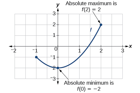
Figure 1.3.9: An absolute minimum at \((0,\, -2)\) and an absolute maximum at \((2,\, 2)\).
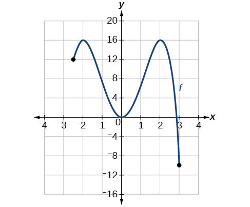
Figure 1.3.10: The graph of \(f\) for Example 1.3.38.
For the function \(f\), find all absolute maxima and minima.
Solution
Observe the graph of \(f.\) The graph attains an absolute maximum in two locations, \(x = -2\) and \(x = 2,\) because at these locations, the graph attains its highest point on the domain of the function. The absolute maximum is the \(y\)-coordinate at \(x = -2\) and \(x = 2,\) which is \(16.\)
The graph attains an absolute minimum at \(x = 3,\) because it is the lowest point on the domain of the function’s graph. The absolute minimum is the \(y\)-coordinate at \(x = 3,\) which is \(-10.\)
1.3.7 Summary
- Average rate of change of a function \(f\) over \([a, b]\) is \(\dfrac{f(b) - f(a)}{b - a}\) — the slope of the secant line through \((a, f(a))\) and \((b, f(b))\).
- The difference quotient \(\dfrac{f(x + h) - f(x)}{h}\) is the average rate of change near \(x\). Computing it requires careful algebra: expand-and-factor for polynomials, common denominators for rational functions, conjugate rationalisation for radicals.
- Increasing / decreasing / constant. A function is increasing on an interval where its outputs grow as inputs grow, decreasing where they shrink, constant where they don’t change.
- Local extrema. A local maximum is an output value larger than all nearby outputs; a local minimum is smaller than all nearby outputs.
- Absolute extrema. The absolute maximum / minimum are the largest / smallest output values across the entire domain.