4.4 Building the Model: Optimization Word Problems

In Section 4.3, we found global extrema of functions that were already given to us. In practice, the function is rarely handed over ready-made. A biologist asks, “What population level maximizes sustainable harvest?” A manufacturer asks, “What dimensions minimize material cost?” The challenge is not just the calculus — it is translating the real-world problem into a mathematical function, identifying the correct domain, and interpreting the answer in context.

4.4.1 The Modeling Process

Problem-Solving Strategy 4.4.1 — Optimization Modeling

To solve an applied optimization problem:

Identify the variables. Assign letters to the quantities involved. Draw a diagram if geometry is involved.
Write the objective function. Express the quantity to be maximized or minimized as a function of the variables.
Use constraints to reduce to one variable. If the objective function involves two or more variables, use the given constraints (equations relating the variables) to eliminate all but one.
Determine the domain. What values of the remaining variable are physically meaningful? Is the interval closed, open, or unbounded?
Optimize and interpret. Find the global maximum or minimum using the methods of Section 4.3 (closed interval method or boundary analysis). State the answer in the context of the original problem, with units.

The domain step is often the most subtle. A physical constraint like “length must be positive” gives an open domain. A constraint like “price between $0 and $35” gives a closed domain. The type of domain determines which method from Section 4.3 to apply. The examples below walk through the full process in several applied contexts.

4.4.2 Closed-Domain Problems

When the domain is a closed interval, the Extreme Value Theorem guarantees that global extrema exist, and the closed interval method (Problem-Solving Strategy 4.3.5) finds them. The challenge is setting up the function and identifying the interval.

Example 4.4.2 — Maximum Sustainable Harvest

A wildlife biologist models the weekly growth rate of a deer population in a nature preserve as

\[G(x) = 0.5x\left(1 - \frac{x}{200}\right) \text{ deer per week}\]

where $x$ is the current population. The preserve can support at most $200$ deer (the carrying capacity). To maintain a stable population, rangers can remove exactly $G(x)$ deer per week — the maximum sustainable harvest at population level $x$. What population level allows the largest sustainable harvest?

Solution (click to reveal)

Step 1. Identify variables. $x$ = current deer population, $G(x)$ = growth rate (deer/week).

Step 2. Objective function. We want to maximize $G(x) = 0.5x\left(1 - \frac{x}{200}\right)$.

Expanding: $G(x) = 0.5x - \frac{x^2}{400} = 0.5x - 0.0025x^2$.

Step 3. Constraints. Already a single-variable function.

Step 4. Domain. The population satisfies $0 \leq x \leq 200$ (no negative populations, and the preserve cannot sustain more than 200). Domain: $[0,\, 200]$.

Step 5. Optimize.

\[G'(x) = 0.5 - 0.005x = 0 \implies x = 100\]

Evaluate at the critical point and endpoints:

$x$	$0$	$100$	$200$
$G(x)$	$0$	$25$	$0$

$G(100) = 0.5(100)(1 - 0.5) = 25$. The figure below shows the growth rate curve.

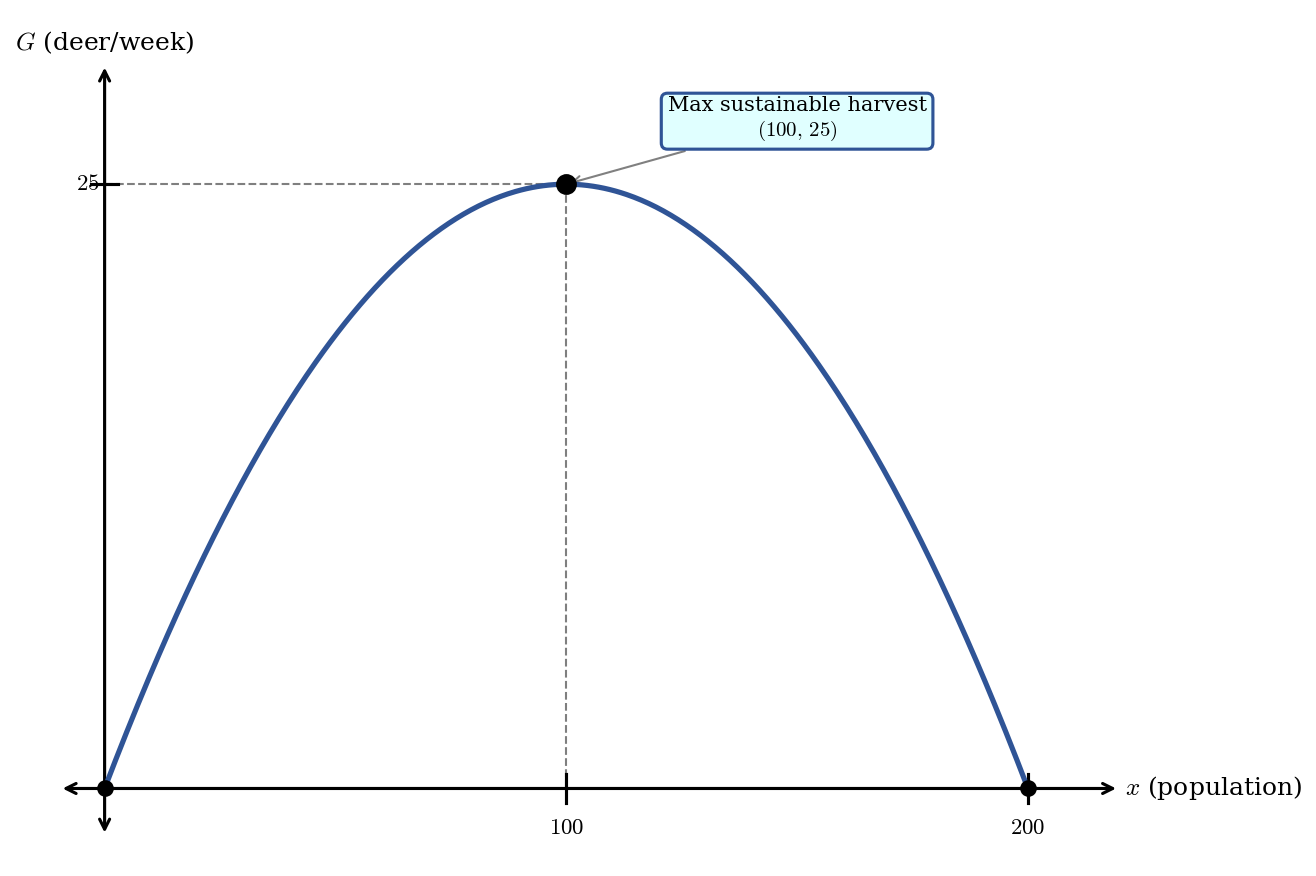
A downward-opening parabola representing the growth rate function G of x, starting at the origin, peaking at x equals 100 with G equals 25, and returning to zero at x equals 200.

Figure: Growth rate $G(x) = 0.5x(1 - x/200)$, with maximum sustainable harvest of $25$ deer per week at population $x = 100$.

Interpretation. The maximum sustainable harvest is 25 deer per week, achieved when the population is maintained at 100 deer — exactly half the carrying capacity. This is a general result in population ecology: for logistic growth, maximum sustainable yield always occurs at half the carrying capacity.

The sustainable harvest example involved a simple quadratic. The next example requires setting up the function from a word description, which introduces an extra layer of modeling.

Example 4.4.3 — Maximizing Revenue

A ride-share company completes $8{,}000$ rides daily at $15 per ride. Market research shows that for each $1 price increase, the company loses $400$ rides; for each $1 decrease, it gains $400$ rides. What price per ride maximizes daily revenue?

Solution (click to reveal)

Step 1. Identify variables. Let $p$ = price per ride (dollars).

Step 2. Objective function. Revenue = price $\times$ quantity. The number of rides depends on price:

\[\text{Rides per day} = 8{,}000 - 400(p - 15) = 14{,}000 - 400p\]

The baseline is $8{,}000$ rides at $p = 15$, adjusted by $-400$ for each dollar above $15 (or $+400$ for each dollar below).

\[R(p) = p(14{,}000 - 400p) = 14{,}000p - 400p^2\]

Step 3. Constraints. Already a single-variable function.

Step 4. Domain. Price must be non-negative: $p \geq 0$. Rides must be non-negative: $14{,}000 - 400p \geq 0$ requires $p \leq 35$. Domain: $[0,\, 35]$.

Step 5. Optimize.

\[R'(p) = 14{,}000 - 800p = 0 \implies p = 17.50\]

Evaluate at the critical point and endpoints:

$p$	$0$	$17.50$	$35$
$R(p)$	$0$	$122{,}500$	$0$

The figure below shows the revenue function.

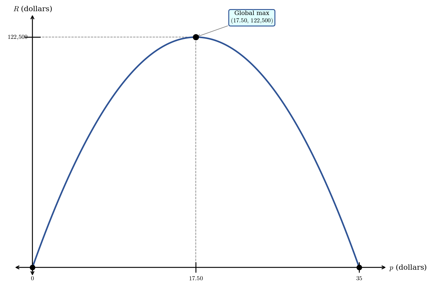
A downward-opening parabola showing revenue R of p as a function of price, starting at the origin, peaking at p equals 17.50 with R equals 122500, and returning to zero at p equals 35.

Figure: $R(p) = 14{,}000p - 400p^2$ showing maximum revenue at $p = 17.50$.

Interpretation. Maximum daily revenue of $122,500 occurs at a price of $17.50 per ride. At this price, the company completes $14{,}000 - 400(17.50) = 7{,}000$ rides daily.

Check: $17.50 \times 7{,}000 = 122{,}500$. $\checkmark$

Checkpoint 4.4.4 — Closed-Domain Modeling Practice

A concert venue can sell tickets at price $p$ dollars. At $p = 50$, they sell $2{,}000$ tickets. For each $5 increase in price, $100$ fewer tickets are sold (and vice versa). What ticket price maximizes revenue?

Hint: Express the number of tickets as a function of $p$, form $R(p) = p \times \text{(tickets)}$, find the domain, and apply the closed interval method.

Solution (click to reveal)

Tickets sold: $2{,}000 - 20(p - 50) = 3{,}000 - 20p$. Revenue: $R(p) = p(3{,}000 - 20p) = 3{,}000p - 20p^2$.

Domain: $p \geq 0$ and $3{,}000 - 20p \geq 0$ gives $p \leq 150$. So $p \in [0,\, 150]$.

$R'(p) = 3{,}000 - 40p = 0$ gives $p = 75$.

$R(0) = 0$, $R(75) = 75(3{,}000 - 1{,}500) = 112{,}500$, $R(150) = 0$.

Maximum revenue: $112,500 at $75 per ticket.

4.4.3 Open- and Unbounded-Domain Problems

Many real-world optimization problems have domains that are open or unbounded. A radius must be positive ($r > 0$), but there is no upper bound imposed by the problem itself. In these cases, the closed interval method does not directly apply, and we must analyze boundary behavior using the techniques from Section 4.3.4: compute limits at the boundaries and verify that the critical point gives a true global extremum.

Example 4.4.5 — Minimizing Material Cost

A company manufactures cylindrical cans that must hold $500$ cm$^3$. The material for the top and bottom costs $0.02/cm$^2$; the material for the curved side costs $0.01/cm$^2$. What dimensions minimize the total material cost?

Solution (click to reveal)

Step 1. Identify variables. Let $r$ = radius (cm) and $h$ = height (cm) of the cylinder, as shown in the figure below.

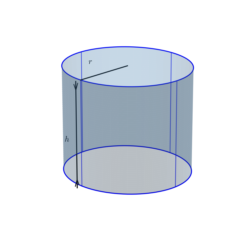
A three-dimensional cylinder with radius r labeled on the top circle and height h labeled along the side.

Figure: Cylinder with radius $r$ and height $h$.

Step 2. Objective function. The total cost combines the top/bottom circles and the rectangular side:

\[C = \underbrace{0.02 \cdot 2\pi r^2}_{\text{top + bottom}} + \underbrace{0.01 \cdot 2\pi r h}_{\text{side}} = 0.04\pi r^2 + 0.02\pi r h\]

Step 3. Reduce to one variable. The volume constraint $\pi r^2 h = 500$ gives $h = \frac{500}{\pi r^2}$. Substituting:

\[C(r) = 0.04\pi r^2 + 0.02\pi r \cdot \frac{500}{\pi r^2} = 0.04\pi r^2 + \frac{10}{r}\]

Step 4. Domain. The radius must be positive: $r > 0$. There is no upper bound — the domain is $(0,\, \infty)$.

Step 5. Optimize. Analyze the boundary behavior first:

As $r \to 0^+$: the term $\frac{10}{r} \to \infty$ (a tiny radius means a very tall, expensive can).
As $r \to \infty$: the term $0.04\pi r^2 \to \infty$ (a huge radius means enormous top/bottom disks).

Since $C(r) \to \infty$ at both ends of the domain, any critical point in between must give a global minimum.

\[C'(r) = 0.08\pi r - \frac{10}{r^2} = 0\]

Multiplying both sides by $r^2$:

\[0.08\pi r^3 = 10 \implies r^3 = \frac{10}{0.08\pi} = \frac{125}{\pi} \implies r = \left(\frac{125}{\pi}\right)^{1/3} \approx 3.41 \text{ cm}\]

Then $h = \frac{500}{\pi(3.41)^2} \approx 13.69$ cm. The figure below shows the cost function.

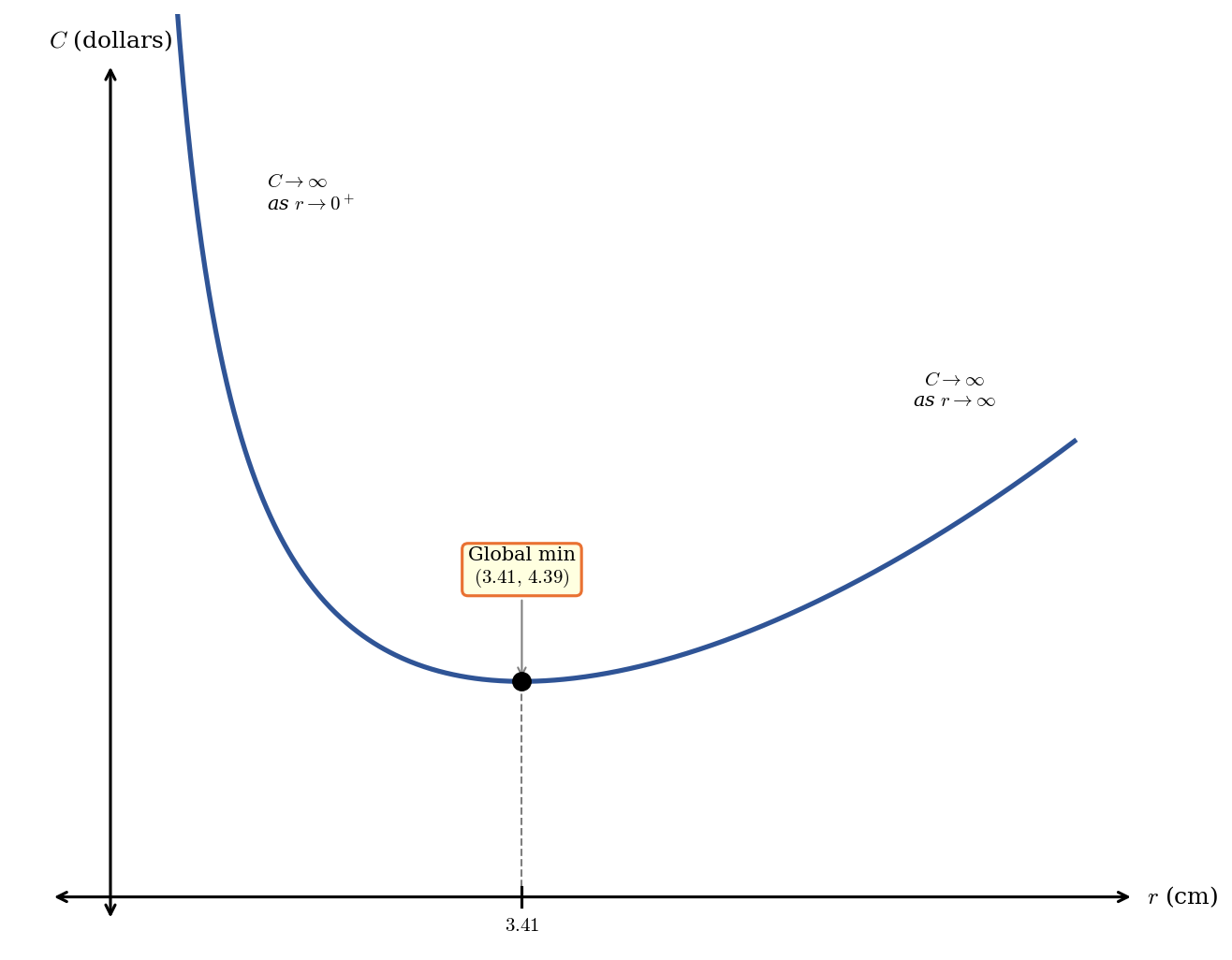
U-shaped curve of the cost function C of r, decreasing steeply from the left as r approaches zero, reaching a minimum near r equals 3.41, then increasing gradually as r grows large.

Figure: $C(r) = 0.04\pi r^2 + 10/r$ with global minimum near $r = 3.41$.

Interpretation. Minimum material cost occurs at $r \approx 3.4$ cm and $h \approx 13.7$ cm. The can is about $4$ times as tall as it is wide — reasonable, since the side material is cheaper than the top and bottom.

Check: Volume $= \pi(3.41)^2(13.69) \approx 500$ cm$^3$. $\checkmark$

In the cylinder example, the cost blows up at both boundaries ($r \to 0^+$ and $r \to \infty$), which guaranteed a minimum in between. The next example features a different boundary pattern: the function starts at zero, rises to a peak, and then decays back toward zero.

Example 4.4.6 — Optimal Foraging Distance

An ecologist studying honeybee colonies models the net energy gain from a foraging trip of distance $r$ kilometers as

\[N(r) = 50\sqrt{r} - 20r, \quad r > 0\]

The term $50\sqrt{r}$ represents the energy collected from flowers (which increases with range but at a diminishing rate), while $20r$ accounts for the flight energy cost (proportional to distance). What foraging distance maximizes the colony’s net energy gain per trip?

Solution (click to reveal)

Step 1. Identify variables. $r$ = foraging distance (km), $N(r)$ = net energy gain (kJ).

Step 2–3. Objective function. Already given as a single-variable function: $N(r) = 50r^{1/2} - 20r$.

Step 4. Domain. Distance must be positive: $r > 0$. (At $r = 0$ the bees stay home and gain nothing.) Domain: $(0,\, \infty)$.

Step 5. Optimize. Analyze boundary behavior:

As $r \to 0^+$: $N(r) \to 0$ (no distance means no gain).
As $r \to \infty$: the linear cost $20r$ dominates the square root term $50\sqrt{r}$, so $N(r) \to -\infty$. (Very long trips cost more energy than they return.)

Find the critical point:

\[N'(r) = \frac{25}{\sqrt{r}} - 20 = 0 \implies \sqrt{r} = \frac{25}{20} = \frac{5}{4} \implies r = \frac{25}{16} = 1.5625 \text{ km}\]

Evaluate:

\[N\!\left(\frac{25}{16}\right) = 50 \cdot \frac{5}{4} - 20 \cdot \frac{25}{16} = 62.5 - 31.25 = 31.25 \text{ kJ}\]

Since $N(r) \to 0$ as $r \to 0^+$ and $N(r) \to -\infty$ as $r \to \infty$, and $r = 25/16$ is the only critical point, this critical point gives the global maximum. The figure below shows the net energy curve.

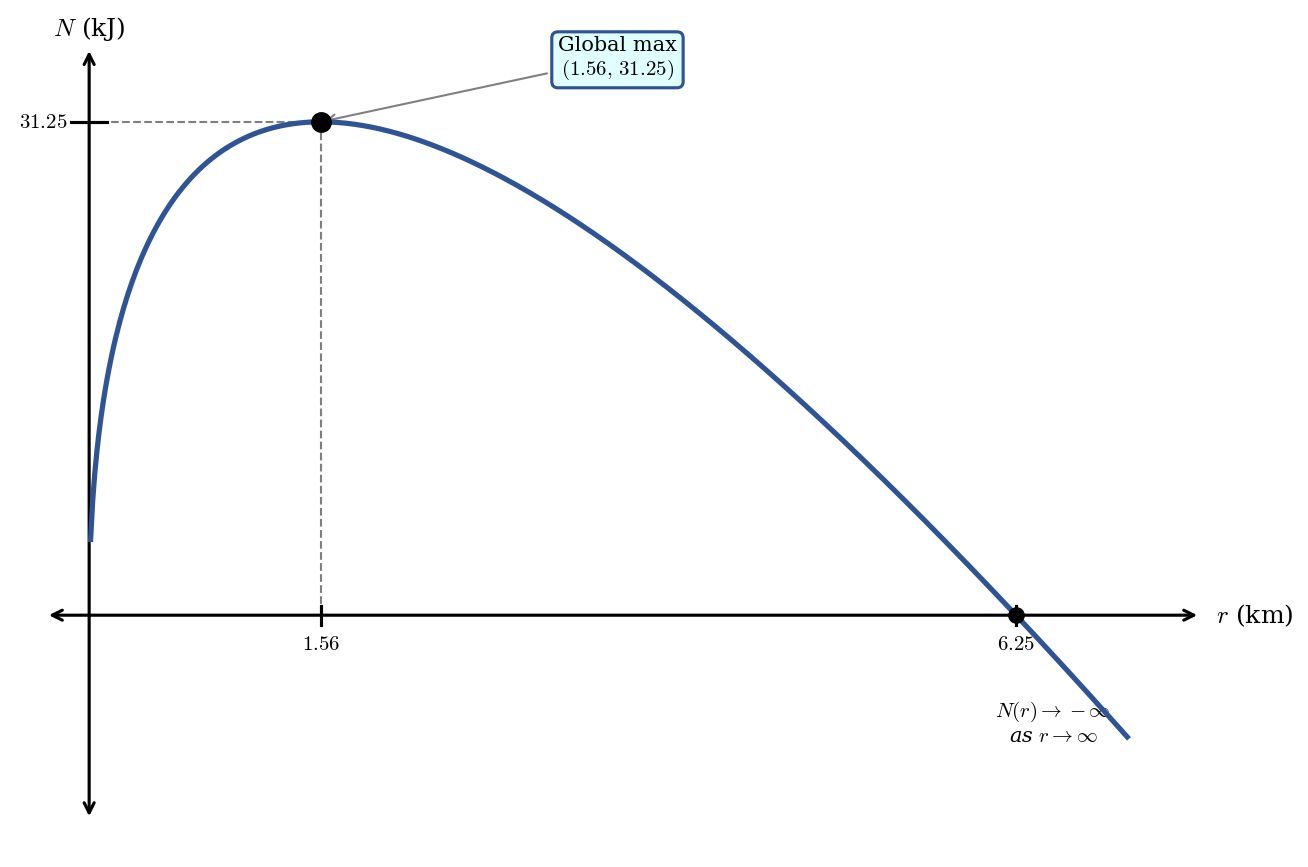
Graph of net energy gain N of r, rising from the origin to a peak at r equals 1.5625 km with N equals 31.25 kJ, then declining through zero and continuing downward.

Figure: $N(r) = 50\sqrt{r} - 20r$ with maximum net energy at $r \approx 1.56$ km.

Interpretation. The optimal foraging distance is approximately $1.56$ km, yielding a net energy gain of $31.25$ kJ per trip. Trips shorter than this do not collect enough nectar; trips longer than this waste more energy in flight than they recover.

Checkpoint 4.4.7 — Open-Domain Modeling Practice

An ecologist is building a rectangular outdoor enclosure along a riverbank (needing fencing on only three sides). With $100$ meters of fencing available, what dimensions maximize the enclosed area?

Hint: Let $x$ be the width (the two sides perpendicular to the river). Then the length along the river is $100 - 2x$, and the area is $A(x) = x(100 - 2x)$.

Solution (click to reveal)

$A(x) = 100x - 2x^2$ for $0 < x < 50$.

$A'(x) = 100 - 4x = 0$ gives $x = 25$. Then the length is $100 - 50 = 50$ m.

$A(25) = 25(50) = 1{,}250$ m$^2$. Since $A(0) = A(50) = 0$ and $A(25) = 1{,}250$, this is the global maximum.

Maximum area: $1{,}250$ m$^2$, with dimensions $25$ m $\times$ $50$ m.

4.4.4 Summary

The optimization modeling process translates a word problem into calculus: identify variables, write the objective function, reduce to one variable using constraints, determine the domain, optimize, and interpret.
Closed-domain problems (finite interval $[a,\, b]$) are solved by the closed interval method: evaluate at critical points and endpoints, then compare.
Open- or unbounded-domain problems require boundary analysis. Compute limits at the edges of the domain to determine whether the function grows without bound or approaches a finite value. A single critical point between two unfavorable boundaries must be the global extremum.
Always interpret the answer in context with appropriate units, and verify that the result is physically reasonable.