4.3 The Best Possible: Global Optimization
After taking a medication, the drug concentration in a patient’s bloodstream rises, peaks, then fades. What dosage timing produces the maximum therapeutic effect? A company knows that raising prices reduces sales — what price maximizes revenue? A biologist managing a fishery wants to maximize sustainable yield. Each question asks: where does a function achieve its best possible value? In Sections 4.1–4.2, we found local extrema — peaks and valleys relative to nearby points. Now we tackle the global picture: finding the absolute best value across the entire domain.
4.3.1 Global vs. Local Extrema
A local maximum is a peak relative to nearby points, but a function may have several such peaks at different heights. The global maximum is the highest of them all.
The key word in this definition is all. A local maximum only needs to beat nearby values; a global maximum must beat every value in the entire domain. Every global extremum is also a local extremum, but the converse is not true — a function may have several local peaks at different heights, and only the tallest qualifies as the global maximum. (It is also possible for a global maximum to be attained at more than one point.) Figure 4.3.2 illustrates this distinction.
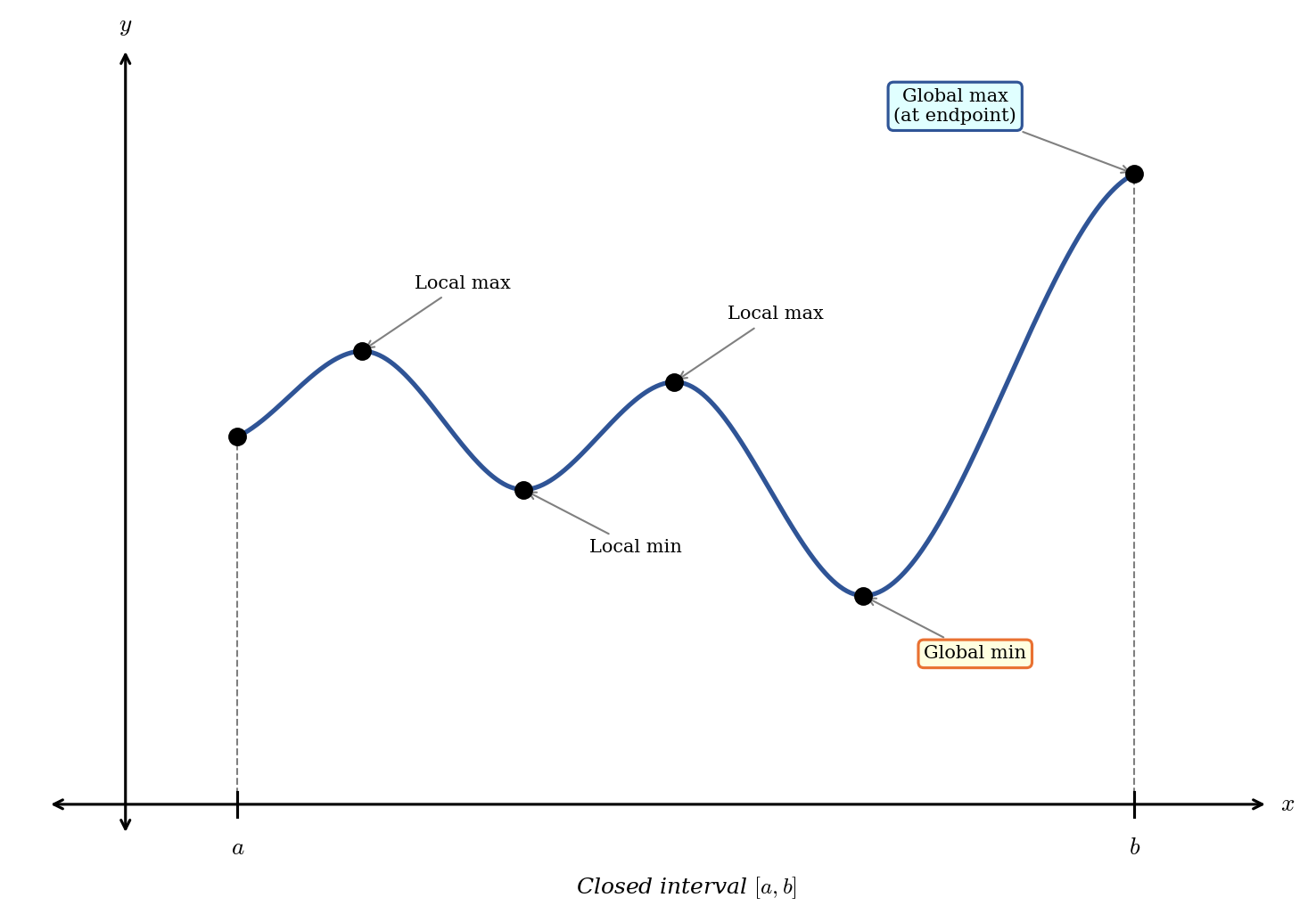
Figure 4.3.2: A continuous function on \([a,\, b]\) showing local maxima, local minima, a global maximum (at an endpoint), and a global minimum (at an interior critical point).
Notice that in Figure 4.3.2, the global maximum occurs at an endpoint, not at one of the interior peaks. This is an important lesson: endpoints are always candidates for global extrema, even if the derivative is not zero there.
The following warmup example applies the definition directly.
4.3.2 The Extreme Value Theorem
Do global extrema always exist? Not necessarily. The function \(f(x) = x^2\) on \((-\infty,\, \infty)\) grows without bound in both directions — it has no global maximum. The function \(g(x) = 1/x\) on \((0,\, 1)\) approaches infinity near \(x = 0\) and never actually reaches its “boundary” value — it has no global minimum on this open interval.
These failures share a common thread: either the domain is not closed or the function is not continuous. The Extreme Value Theorem guarantees that both problems disappear when these two conditions are met.
The theorem does not tell us where the extrema occur — only that they exist. To locate them, we need to narrow the search. By Fermat’s Theorem (from Section 4.1), if \(f\) has a local extremum at an interior point \(c\), then either \(f'(c) = 0\) or \(f'(c)\) does not exist. Since every global extremum is either a local extremum or an endpoint, the candidates for global extrema are precisely the critical points inside \((a,\, b)\) together with the endpoints \(a\) and \(b\). This observation gives us a systematic procedure.
4.3.3 The Closed Interval Method
This method is powerful because it reduces an infinite search (check every point in \([a,\, b]\)) to a finite one (check only critical points and endpoints). The next example demonstrates the method on a polynomial.
Find the global maximum and minimum of \(f(x) = 2x^3 + 3x^2 - 12x + 4\) on \([-4,\, 2]\).
Solution (click to reveal)
Step 1. Find critical points:
\[f'(x) = 6x^2 + 6x - 12 = 6(x^2 + x - 2) = 6(x + 2)(x - 1) = 0\]
This gives \(x = -2\) and \(x = 1\). Both lie in the open interval \((-4,\, 2)\), so both are candidates.
Step 2. Evaluate \(f\) at the critical points and endpoints:
| \(x\) | \(-4\) | \(-2\) | \(1\) | \(2\) |
|---|---|---|---|---|
| \(f(x)\) | \(-28\) | \(24\) | \(-3\) | \(8\) |
The computations: \(f(-4) = 2(-64) + 3(16) - 12(-4) + 4 = -128 + 48 + 48 + 4 = -28\). Similarly, \(f(-2) = -16 + 12 + 24 + 4 = 24\), \(f(1) = 2 + 3 - 12 + 4 = -3\), and \(f(2) = 16 + 12 - 24 + 4 = 8\).
Step 3. Compare values. The figure below shows the graph of \(f\).
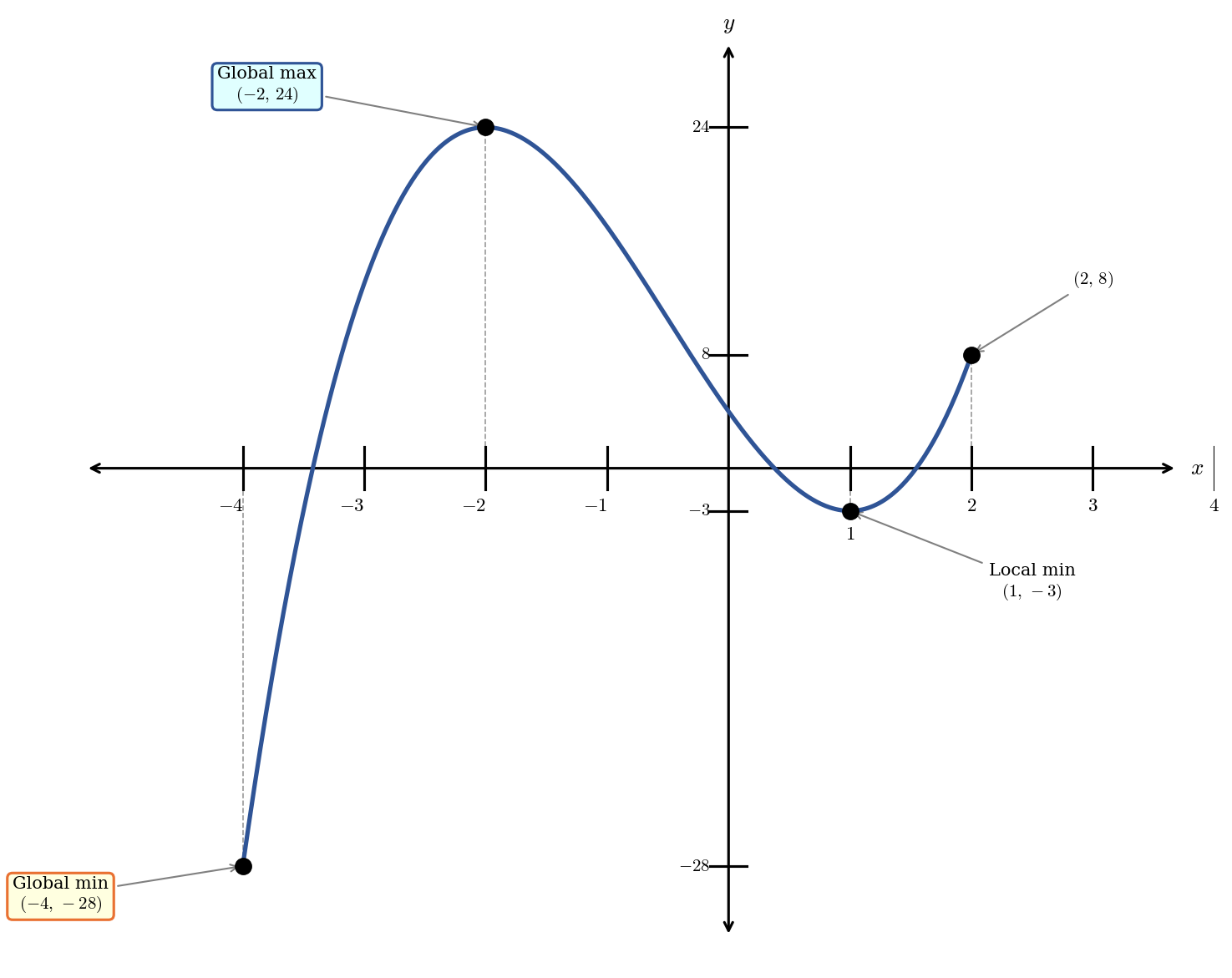
Figure: \(f(x) = 2x^3 + 3x^2 - 12x + 4\) on \([-4,\, 2]\), showing the global max at \((-2,\, 24)\) and global min at \((-4,\, -28)\).
Global maximum: \(24\) at \(x = -2\). Global minimum: \(-28\) at \(x = -4\).
Notice that the global minimum occurs at an endpoint, not at a critical point. The closed interval method catches this because it always checks both endpoints.
In Example 4.3.6, both critical points fell inside the interval. In practice, this does not always happen — a critical point may lie outside the interval of interest, in which case we simply discard it. The next two examples illustrate this important situation.
When all critical points fall outside the interval, the function must be monotonic (entirely increasing or entirely decreasing) throughout. In that case, the global extrema occur at the endpoints. The next example features a quotient, where one critical point is inside the interval and another falls outside.
The lesson from Examples 4.3.7 and 4.3.8 is clear: always check whether each critical point actually belongs to the interval before including it in the candidate list.
4.3.4 Optimization on Unbounded Domains
The Extreme Value Theorem requires a closed interval \([a,\, b]\). When the domain is unbounded — like \([0,\, \infty)\) — or open — like \((0,\, \infty)\) — the theorem does not apply, and global extrema are not guaranteed to exist. A function might climb forever, or approach a value without ever reaching it.
To handle these cases, we need to analyze what happens at the boundaries of the domain. There are three tools for this analysis:
Compute limits. Evaluate \(\lim_{x \to \infty} f(x)\), \(\lim_{x \to -\infty} f(x)\), or \(\lim_{x \to a^+} f(x)\) as appropriate. If a limit is \(\pm\infty\), the function grows or falls without bound in that direction and cannot attain a global extremum there.
Check the derivative’s sign. If \(f'(x) > 0\) throughout the domain, \(f\) is always increasing and has no interior peaks. If \(f'(x) < 0\) throughout, \(f\) is always decreasing. A sign change in \(f'\) indicates a local extremum.
Use the graph for confirmation. After the algebraic analysis, sketching the function (or using the graph of \(f'\)) confirms the behavior visually.
The following principle covers the most common situation in applications.
One-critical-point principle. If \(f\) is continuous on an interval, has exactly one critical point \(c\) in the interior, and the function values at the boundaries (endpoints or limits at \(\pm\infty\)) are both less than \(f(c)\), then \(f(c)\) is the global maximum. Similarly, if the boundary values are both greater than \(f(c)\), then \(f(c)\) is the global minimum.
The next example demonstrates these tools on a simple function where the critical point falls outside the domain.
Find the global extrema of \(f(t) = 3 - 4t - 2t^2\) on \([0,\, \infty)\).
Solution (click to reveal)
Step 1. Find critical points.
\[f'(t) = -4 - 4t = -4(1 + t) = 0 \implies t = -1\]
Since \(t = -1 \notin [0,\, \infty)\), there are no critical points in the domain.
Step 2. Evaluate at the endpoint. The domain has one finite endpoint:
\[f(0) = 3\]
Step 3. Analyze the boundary behavior. As \(t \to \infty\), the \(-2t^2\) term dominates:
\[\lim_{t \to \infty} f(t) = \lim_{t \to \infty} (3 - 4t - 2t^2) = -\infty\]
The function decreases without bound — it has no floor to land on.
Step 4. Draw the conclusion. Since \(f'(t) = -4(1 + t) < 0\) for all \(t \geq 0\), the function is strictly decreasing on \([0,\, \infty)\). The largest value occurs at the left endpoint, and the function never reaches a smallest value because it falls toward \(-\infty\).
The figure below confirms this: the curve starts at \((0,\, 3)\) and decreases steadily.
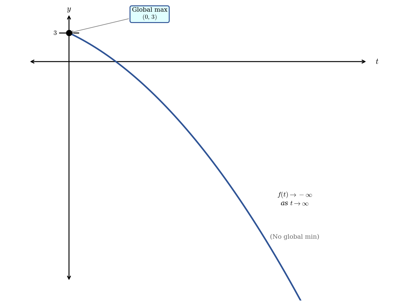
Figure: \(f(t) = 3 - 4t - 2t^2\) on \([0,\, \infty)\). Global max at \((0,\, 3)\); no global min.
Global maximum: \(3\) at \(t = 0\). No global minimum (the function decreases without bound).
The next example features a function with a critical point inside the unbounded domain. The analysis is richer because we must compare the critical value against both the endpoint and the long-term behavior.
The concentration of a drug in the bloodstream \(t\) hours after administration is modeled by
\[C(t) = 20t \cdot e^{-0.4t} \quad \text{mg/L}, \quad t \geq 0\]
When does the maximum concentration occur, and what is it?
Solution (click to reveal)
Step 1. Find critical points. Using the product rule:
\[C'(t) = 20 e^{-0.4t} + 20t(-0.4)e^{-0.4t} = 20e^{-0.4t}(1 - 0.4t)\]
Since \(e^{-0.4t} > 0\) for all \(t\), we set \(1 - 0.4t = 0\), giving \(t = 2.5\) hours.
Step 2. Evaluate at the endpoint and critical point.
\[C(0) = 0 \qquad C(2.5) = 20(2.5)e^{-1} = 50e^{-1} \approx 18.4 \text{ mg/L}\]
Step 3. Analyze the long-term behavior. As \(t \to \infty\), the exponential decay \(e^{-0.4t}\) shrinks to zero much faster than the linear factor \(20t\) grows. Formally:
\[\lim_{t \to \infty} 20t \cdot e^{-0.4t} = 0\]
This can be confirmed by evaluating \(C\) at a few large values: \(C(10) \approx 3.7\), \(C(20) \approx 0.07\), \(C(30) \approx 0.0004\). The concentration approaches zero as the drug is metabolized.
Step 4. Draw the conclusion. We have:
- At the left boundary: \(C(0) = 0\)
- At the critical point: \(C(2.5) \approx 18.4\)
- At the right boundary (\(t \to \infty\)): \(C(t) \to 0\)
Since \(C(2.5)\) exceeds both boundary values, and \(t = 2.5\) is the only critical point, \(C(2.5)\) is the global maximum. The figure below shows the concentration curve.
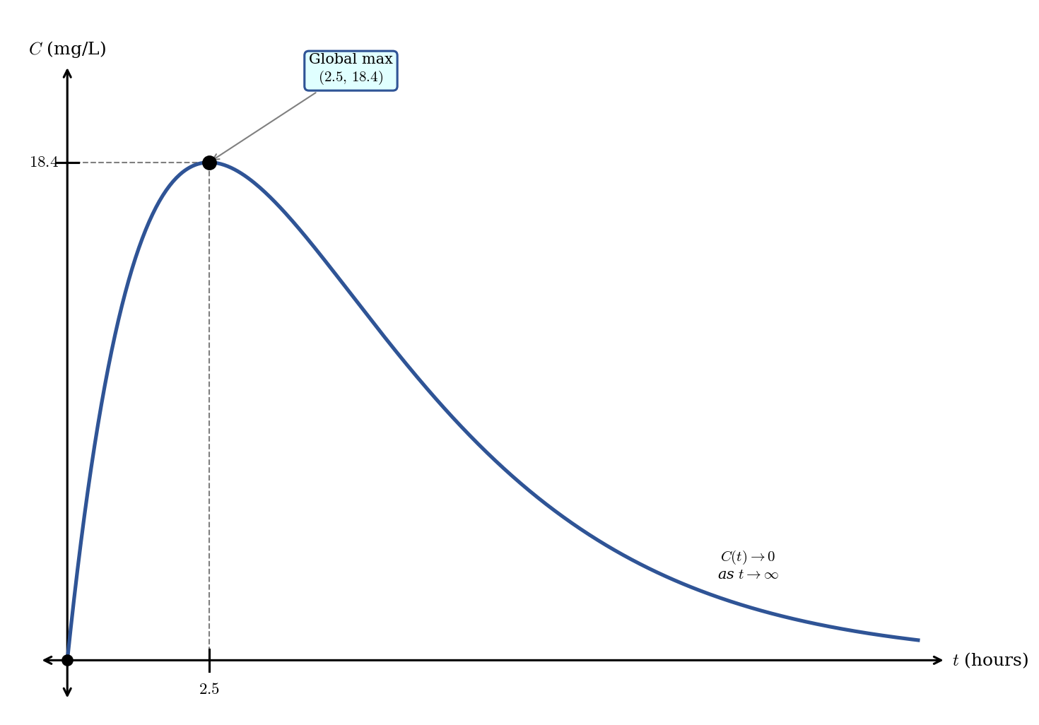
Figure: \(C(t) = 20te^{-0.4t}\) showing peak concentration at \(t = 2.5\) hours.
Global maximum: approximately \(18.4\) mg/L at \(t = 2.5\) hours. Global minimum: \(0\) mg/L at \(t = 0\) (and approached again as \(t \to \infty\), though never quite reached for \(t > 0\)).
In a clinical setting, this tells a pharmacist that the drug reaches its peak effect \(2.5\) hours after administration.
4.3.5 Summary
Global extrema are the absolute largest and smallest values of a function over its entire domain.
The Extreme Value Theorem guarantees that a continuous function on a closed interval \([a,\, b]\) attains both a global maximum and a global minimum.
The Closed Interval Method reduces the search to a finite candidate list: evaluate \(f\) at all critical points in \((a,\, b)\) and at both endpoints, then compare. Critical points outside the interval are discarded.
On unbounded or open domains, the EVT does not apply. Analyze boundary behavior using limits, the sign of \(f'\), and graphs. If the function has a single critical point and the boundary values are both less favorable, that critical point yields the global extremum.