3.1 Defining the Derivative
Now that we have both a conceptual understanding of a limit and the practical ability to compute limits, we have established the foundation for our study of calculus, the branch of mathematics in which we compute derivatives and integrals. Most mathematicians and historians agree that calculus was developed independently by the Englishman Isaac Newton \(\text{(1643–1727)}\) and the German Gottfried Leibniz \(\text{(1646–1716),}\) whose images appear in Figure 1. When we credit Newton and Leibniz with developing calculus, we are really referring to the fact that Newton and Leibniz were the first to understand the relationship between the derivative and the integral. Both mathematicians benefited from the work of predecessors, such as Barrow, Fermat, and Cavalieri. The initial relationship between the two mathematicians appears to have been amicable; however, in later years a bitter controversy erupted over whose work took precedence. Although it seems likely that Newton did, indeed, arrive at the ideas behind calculus first, we are indebted to Leibniz for the notation that we commonly use today.

Figure 1 Newton and Leibniz are credited with developing calculus independently.
3.1.1 Tangent Lines
We begin our study of calculus by revisiting the notion of secant lines and tangent lines. Recall that we used the slope of a secant line to a function at a point \((a,f(a))\) to estimate the rate of change, or the rate at which one variable changes in relation to another variable. We can obtain the slope of the secant by choosing a value of \(x\) near \(a\) and drawing a line through the points \((a,f(a))\) and \(\left( {x,f(x)} \right),\) as shown in Figure 2. The slope of this line is given by an equation in the form of a difference quotient:
\[m_{\text{sec}} = \frac{f(x) - f(a)}{x - a}. \tag{1}\]
We can also calculate the slope of a secant line to a function at a value \(a\) by using this equation and replacing \(x\) with \(a + h,\) where \(h\) is a value close to 0. We can then calculate the slope of the line through the points \((a,f(a))\) and \((a + h,f\left( {a + h} \right)).\) In this case, we find the secant line has a slope given by the following difference quotient with increment \(h\text{:}\)
\[m_{\text{sec}} = \frac{f\left( {a + h} \right) - f(a)}{a + h - a} = \frac{f\left( {a + h} \right) - f(a)}{h}. \tag{2}\]
These two expressions for calculating the slope of a secant line are illustrated in Figure 2. We will see that each of these two methods for finding the slope of a secant line is of value. Depending on the setting, we can choose one or the other. The primary consideration in our choice usually depends on ease of calculation.
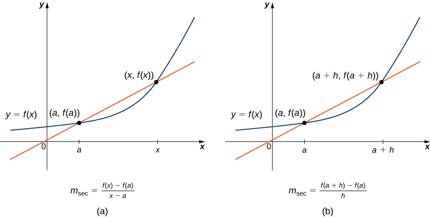
Figure 2 We can calculate the slope of a secant line in either of two ways.
In Figure 3(a) we see that, as the values of \(x\) approach \(a,\) the slopes of the secant lines provide better estimates of the rate of change of the function at \(a.\) Furthermore, the secant lines themselves approach the tangent line to the function at \(a,\) which represents the limit of the secant lines. Similarly, Figure 3(b) shows that as the values of \(h\) get closer to \(0,\) the secant lines also approach the tangent line. The slope of the tangent line at \(a\) is the rate of change of the function at \(a,\) as shown in Figure 3(c).
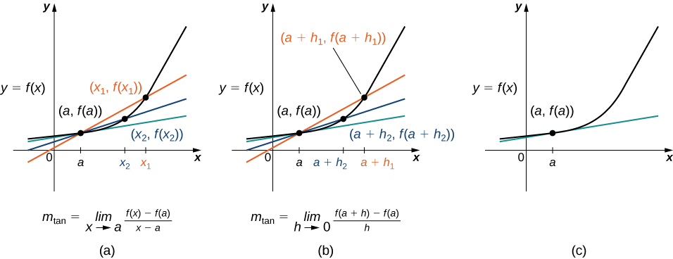
Figure 3 The secant lines approach the tangent line (shown in green) as the second point approaches the first.
In Figure 4 we show the graph of \(f(x) = \sqrt{x}\) and its tangent line at \((1,1)\) in a series of tighter intervals about \(x = 1.\) As the intervals become narrower, the graph of the function and its tangent line appear to coincide, making the values on the tangent line a good approximation to the values of the function for choices of \(x\) close to \(1.\) In fact, the graph of \(f(x)\) itself appears to be locally linear in the immediate vicinity of \(x = 1.\)
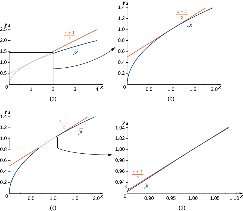
Figure 4 For values of \(x\) close to \(1,\) the graph of \(f(x) = \sqrt{x}\) and its tangent line appear to coincide.
Formally we may define the tangent line to the graph of a function as follows.
Just as we have used two different expressions to define the slope of a secant line, we use two different forms to define the slope of the tangent line. In this text we use both forms of the definition. As before, the choice of definition will depend on the setting. Now that we have formally defined a tangent line to a function at a point, we can use this definition to find equations of tangent lines.
Find an equation of the line tangent to the graph of \(f(x) = x^{2}\) at \(x = 3.\)
Solution (click to reveal)
First find the slope of the tangent line. In this example, use Equation 5.
\[\begin{array}{clccl} m_{\text{tan}} & {= \underset{x\rightarrow 3}{\text{lim}}\frac{f(x) - f(3)}{x - 3}} & & & \text{Apply the definition.} \\ & {= \underset{x\rightarrow 3}{\text{lim}}\frac{x^{2} - 9}{x - 3}} & & & {\text{Substitute}\ f(x) = x^{2}\ \text{and}\ f(3) = 9.} \\ & {= \underset{x\rightarrow 3}{\text{lim}}\frac{\left( {x - 3} \right)\left( {x + 3} \right)}{x - 3} = \underset{x\rightarrow 3}{\text{lim}}\left( {x + 3} \right) = 6} & & & \text{Factor the numerator to evaluate the limit.} \end{array} \tag{7}\]
Next, find a point on the tangent line. Since the line is tangent to the graph of \(f(x)\) at \(x = 3,\) it passes through the point \(\left( {3,f(3)} \right).\) We have \(f(3) = 9,\) so the tangent line passes through the point \(\left( {3,9} \right).\)
Using the point-slope equation of the line with the slope \(m = 6\) and the point \(\left( {3,9} \right),\) we obtain the line \(y - 9 = 6\left( {x - 3} \right).\) Simplifying, we have \(y = 6x - 9.\) The graph of \(f(x) = x^{2}\) and its tangent line at \(3\) are shown in Figure 5.
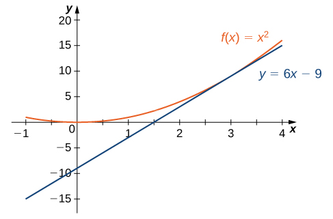
Figure 5 The tangent line to \(f(x)\) at \(x = 3.\)
Find an equation of the line tangent to the graph of \(f(x) = 1\text{/}x\) at \(x = 2.\)
Solution (click to reveal)
We can use Equation 5, but as we have seen, the results are the same if we use Equation 6.
\[\begin{array}{clccl} m_{\text{tan}} & {= \underset{x\rightarrow 2}{\text{lim}}\frac{f(x) - f(2)}{x - 2}} & & & \text{Apply the definition.} \\ & {= \underset{x\rightarrow 2}{\text{lim}}\frac{\frac{1}{x} - \frac{1}{2}}{x - 2}} & & & {\text{Substitute}\ f(x) = \frac{1}{x}\ \text{and}\mspace{2mu} f(2) = \frac{1}{2}.} \\ & {= \underset{x\rightarrow 2}{\text{lim}}\frac{\frac{1}{x} - \frac{1}{2}}{x - 2} \cdot \frac{2x}{2x}} & & & \begin{array}{l} {\text{Multiply numerator and denominator by}\ 2x\ \text{to}} \\ \text{simplify fractions.} \end{array} \\ & {= \underset{x\rightarrow 2}{\text{lim}}\frac{\left( {2 - x} \right)}{\left( {x - 2} \right)\left( {2x} \right)}} & & & \text{Simplify.} \\ & {= \underset{x\rightarrow 2}{\text{lim}}\frac{-1}{2x}} & & & {\text{Simplify using}\ \frac{2 - x}{x - 2} = -1,\text{for}\ x \neq 2.} \\ & {= - \frac{1}{4}} & & & \text{Evaluate the limit.} \end{array} \tag{9}\]
We now know that the slope of the tangent line is \(- \frac{1}{4}.\) To find an equation of the tangent line, we also need a point on the line. We know that \(f(2) = \frac{1}{2}.\) Since the tangent line passes through the point \((2,\frac{1}{2})\) we can use the point-slope equation of a line to find an equation of the tangent line. Thus the tangent line has the equation \(y = - \frac{1}{4}x + 1.\) The graphs of \(f(x) = \frac{1}{x}\) and \(y = - \frac{1}{4}x + 1\) are shown in Figure 6.
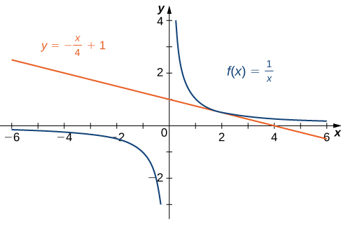
Figure 6 The line is tangent to \(f(x)\) at \(x = 2.\)
3.1.2 The Derivative of a Function at a Point
The type of limit we compute in order to find the slope of the line tangent to a function at a point occurs in many applications across many disciplines. These applications include velocity and acceleration in physics, marginal profit functions in business, and growth rates in biology. This limit occurs so frequently that we give this value a special name: the derivative. The process of finding a derivative is called differentiation.
3.1.3 Velocities and Rates of Change
Now that we can evaluate a derivative, we can use it in velocity applications. Recall that if \(s(t)\) is the position of an object moving along a coordinate axis, the average velocity of the object over a time interval \(\left\lbrack {a,t} \right\rbrack\) if \(t > a\) or \(\left\lbrack {t,a} \right\rbrack\) if \(t < a\) is given by the difference quotient
\[v_{\text{ave}} = \frac{s(t) - s(a)}{t - a}. \tag{14}\]
As the values of \(t\) approach \(a,\) the values of \(v_{\text{ave}}\) approach the value we call the instantaneous velocity at \(a.\) That is, instantaneous velocity at \(a,\) denoted \(v(a),\) is given by
\[v(a) = s'(a) = \underset{t\rightarrow a}{\text{lim}}\frac{s(t) - s(a)}{t - a}. \tag{15}\]
To better understand the relationship between average velocity and instantaneous velocity, see Figure 7. In this figure, the slope of the tangent line (shown in red) is the instantaneous velocity of the object at time \(t = a\) whose position at time \(t\) is given by the function \(s(t).\) The slope of the secant line (shown in green) is the average velocity of the object over the time interval \(\left\lbrack {a,t} \right\rbrack.\)
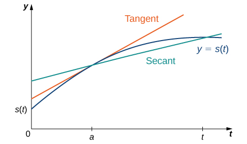
Figure 7 The slope of the secant line is the average velocity over the interval \(\lbrack a,t\rbrack.\) The slope of the tangent line is the instantaneous velocity.
We can use Equation 10 to calculate the instantaneous velocity, or we can estimate the velocity of a moving object by using a table of values. We can then confirm the estimate by using Equation 14.
A lead weight on a spring is oscillating up and down. Its position at time \(t\) with respect to a fixed horizontal line is given by \(s(t) = \text{sin}\ t\) (Figure 8). Use a table of values to estimate \(v(0).\) Check the estimate by using Equation 10.
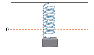
Figure 8 A lead weight suspended from a spring in vertical oscillatory motion.
Solution (click to reveal)
We can estimate the instantaneous velocity at \(t = 0\) by computing a table of average velocities using values of \(t\) approaching \(0,\) as shown in Table 1.
| \(t\) | \(\frac{\text{sin}\mspace{2mu} t - \text{sin}\mspace{2mu} 0}{t - 0} = \frac{\text{sin}\mspace{2mu} t}{t}\) |
|---|---|
| \(-0.1\) | \(0.998334166\) |
| \(-0.01\) | \(0.9999833333\) |
| \(-0.001\) | \(0.999999833\) |
| \(0.001\) | \(0.999999833\) |
| \(0.01\) | \(0.9999833333\) |
| \(0.1\) | \(0.998334166\) |
Table 1 Average velocities using values of \(t\) approaching 0
From the table we see that the average velocity over the time interval \(\left\lbrack {-0.1,0} \right\rbrack\) is \(0.998334166,\) the average velocity over the time interval \(\left\lbrack {-0.01,0} \right\rbrack\) is \(0.9999833333,\) and so forth. Using this table of values, it appears that a good estimate is \(v(0) = 1.\)
By using Equation 10, we can see that
\[v(0) = s'(0) = \underset{t\rightarrow 0}{\text{lim}}\frac{\text{sin}\mspace{2mu} t - \text{sin}\mspace{2mu} 0}{t - 0} = \underset{t\rightarrow 0}{\text{lim}}\frac{\text{sin}\mspace{2mu} t}{t} = 1. \tag{16}\]
Thus, in fact, \(v(0) = 1.\)
As we have seen throughout this section, the slope of a tangent line to a function and instantaneous velocity are related concepts. Each is calculated by computing a derivative and each measures the instantaneous rate of change of a function, or the rate of change of a function at any point along the function.
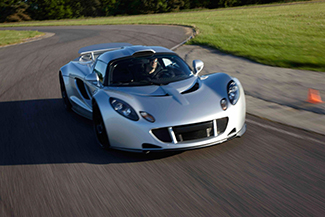
Figure 9 (credit: modification of work by Codex41, Flickr)
Reaching a top speed of \(270.49\) mph, the Hennessey Venom GT is one of the fastest cars in the world. In tests it went from \(0\) to \(60\) mph in \(3.05\) seconds, from \(0\ \text{to}\ 100\) mph in \(5.88\) seconds, from \(0\ \text{to}\ 200\) mph in \(14.51\) seconds, and from \(0\ \text{to}\ 229.9\) mph in \(19.96\) seconds. Use this data to draw a conclusion about the rate of change of velocity (that is, its acceleration) as it approaches \(229.9\) mph. Does the rate at which the car is accelerating appear to be increasing, decreasing, or constant?
Solution (click to reveal)
First observe that \(60\) mph = \(88\) ft/s, \(100\) mph \(\approx 146.67\) ft/s, \(200\) mph \(\approx 293.33\) ft/s, and \(229.9\) mph \(\approx 337.19\) ft/s. We can summarize the information in a table.
| \(t\) | \(v(t)\) |
|---|---|
| \(0\) | \(0\) |
| \(3.05\) | \(88\) |
| \(5.88\) | \(146.67\) |
| \(14.51\) | \(293.33\) |
| \(19.96\) | \(337.19\) |
Table 2 \(v(t)\) at different values of \(t\)
Now compute the average acceleration of the car in feet per second per second on intervals of the form \(\left\lbrack {t,19.96} \right\rbrack\) as \(t\) approaches \(19.96,\) as shown in the following table.
| \(t\) | \(\frac{v(t) - v(19.96)}{t - 19.96} = \frac{v(t) - 337.19}{t - 19.96}\) |
|---|---|
| \(0.0\) | \(16.89\) |
| \(3.05\) | \(14.74\) |
| \(5.88\) | \(13.53\) |
| \(14.51\) | \(8.05\) |
Table 3 Average acceleration
The rate at which the car is accelerating is decreasing as its velocity approaches \(229.9\) mph \(\text{(}337.19\) ft/s).
For the following exercises, use Equation 3 to find the slope of the secant line between the values \(x_{1}\) and \(x_{2}\) for each function \(y = f(x).\)
1. \(f(x) = 4x + 7;x_{1} = 2,x_{2} = 5\)
Solution (click to reveal)
\(4\)
2. \(f(x) = 8x - 3;x_{1} = -1,x_{2} = 3\)
3. \(f(x) = x^{2} + 2x + 1;x_{1} = 3,x_{2} = 3.5\)
Solution (click to reveal)
\(8.5\)
4. \(f(x) = \text{−}x^{2} + x + 2;x_{1} = 0.5,x_{2} = 1.5\)
5. \(f(x) = \frac{4}{3x - 1};x_{1} = 1,x_{2} = 3\)
Solution (click to reveal)
\(- \frac{3}{4}\)
6. \(f(x) = \frac{x - 7}{2x + 1};x_{1} = 0,x_{2} = 2\)
7. \(f(x) = \sqrt{x};x_{1} = 1,x_{2} = 16\)
Solution (click to reveal)
\(0.2\)
8. \(f(x) = \sqrt{x - 9};x_{1} = 10,x_{2} = 13\)
9. \(f(x) = x^{1\text{/}3} + 1;x_{1} = 0,x_{2} = 8\)
Solution (click to reveal)
\(0.25\)
10. \(f(x) = 6x^{2\text{/}3} + 2x^{1\text{/}3};x_{1} = 1,x_{2} = 27\)
For the following functions,
- use Equation 6 to find the slope of the tangent line \(m_{\text{tan}} = f'(a),\) and
- find an equation of the tangent line to \(f\) at \(x = a.\)
11. \(f(x) = 3 - 4x,a = 2\)
Solution (click to reveal)
- \(-4\) b. \(y = 3 - 4x\)
12. \(f(x) = \frac{x}{5} + 6,a = -1\)
13. \(f(x) = x^{2} + x,a = 1\)
Solution (click to reveal)
- \(3\) b. \(y = 3x - 1\)
14. \(f(x) = 1 - x - x^{2},a = 0\)
15. \(f(x) = \frac{7}{x},a = 3\)
Solution (click to reveal)
- \(\frac{-7}{9}\) b. \(y = \frac{-7}{9}x + \frac{14}{3}\)
16. \(f(x) = \sqrt{x + 8},a = 1\)
17. \(f(x) = 2 - 3x^{2},a = -2\)
Solution (click to reveal)
- \(12\) b. \(y = 12x + 14\)
18. \(f(x) = \frac{-3}{x - 1},a = 4\)
19. \(f(x) = \frac{2}{x + 3},a = -4\)
Solution (click to reveal)
- \(-2\) b. \(y = -2x - 10\)
20. \(f(x) = \frac{3}{x^{2}},a = 3\)
For the following functions \(y = f(x),\) find \(f'(a)\) using Equation 10.
21. \(f(x) = 5x + 4,a = -1\)
Solution (click to reveal)
\(5\)
22. \(f(x) = -7x + 1,a = 3\)
23. \(f(x) = x^{2} + 9x,a = 2\)
Solution (click to reveal)
\(13\)
24. \(f(x) = 3x^{2} - x + 2,a = 1\)
25. \(f(x) = \sqrt{x},a = 4\)
Solution (click to reveal)
\(\frac{1}{4}\)
26. \(f(x) = \sqrt{x - 2},a = 6\)
27. \(f(x) = \frac{1}{x},a = 2\)
Solution (click to reveal)
\(- \frac{1}{4}\)
28. \(f(x) = \frac{1}{x - 3},a = -1\)
29. \(f(x) = \frac{1}{x^{3}},a = 1\)
Solution (click to reveal)
\(-3\)
30. \(f(x) = \frac{1}{\sqrt{x}},a = 4\)
For the following exercises, given the function \(y = f(x),\)
- find the slope of the secant line \(PQ\) for each point \(Q\left( {x,f(x)} \right)\) with \(x\) value given in the table.
- Use the answers from a. to estimate the value of the slope of the tangent line at \(P.\)
- Use the answer from b. to find an equation of the tangent line to \(f\) at point \(P.\)
31. [T] \(f(x) = x^{2} + 3x + 4,P\left( {1,8} \right)\) (Round to \(6\) decimal places.)
| \(x\) | Slope \(m_{PQ}\) | \(x\) | Slope \(m_{PQ}\) |
|---|---|---|---|
| 1.1 | 0.9 | ||
| 1.01 | 0.99 | ||
| 1.001 | 0.999 | ||
| 1.0001 | 0.9999 | ||
| 1.00001 | 0.99999 | ||
| 1.000001 | 0.999999 |
Solution (click to reveal)
- \(\text{(i)}\ 5.100000,\) \(\text{(ii)}\ 5.010000,\) \(\text{(iii)}\ 5.001000,\) \(\text{(iv)}\ 5.000100,\) \(\text{(v)}\ 5.000010,\) \(\text{(vi)}\ 5.000001,\) \(\text{(vii)}\ 4.900000,\) \(\text{(viii)}\ 4.990000,\) \(\text{(ix)}\ 4.999000,\) \(\text{(x)}\ 4.999900,\) \(\text{(xi)}\ 4.999990,\) \(\text{(x)}\ 4.999999\) b. \(m_{\text{tan}} = 5\) c. \(y = 5x + 3\)
32. [T] \(f(x) = \frac{x + 1}{x^{2} - 1},P\left( {0,-1} \right)\)
| \(x\) | Slope \(m_{PQ}\) | \(x\) | Slope \(m_{PQ}\) |
|---|---|---|---|
| 0.1 | \(-0.1\) | ||
| 0.01 | \(-0.01\) | ||
| 0.001 | \(-0.001\) | ||
| 0.0001 | \(-0.0001\) | ||
| 0.00001 | \(-0.00001\) | ||
| 0.000001 | \(-0.000001\) |
33. [T] \(f(x) = 10e^{0.5x},P\left( {0,10} \right)\) (Round to \(4\) decimal places.)
| \(x\) | Slope \(m_{PQ}\) |
|---|---|
| \(-0.1\) | |
| \(-0.01\) | |
| \(-0.001\) | |
| \(-0.0001\) | |
| \(-0.00001\) | |
| −0.000001 |
Solution (click to reveal)
- \(\text{(i)}\ 4.8771,\) \(\text{(ii)}\ 4.9875\ \text{(iii)}\ 4.9988,\) \(\text{(iv)}\ 4.9999,\) \(\text{(v)}\ 4.9999,\) \(\text{(vi)}\ 4.9999\) b. \(m_{\text{tan}} = 5\) c. \(y = 5x + 10\)
34. [T] \(f(x) = \text{tan}\mspace{2mu}(x),P\left( {\pi,0} \right)\)
| \(x\) | Slope \(m_{PQ}\) |
|---|---|
| 3.1 | |
| 3.14 | |
| 3.141 | |
| 3.1415 | |
| 3.14159 | |
| 3.141592 |
[T] For the following position functions \(y = s(t),\) an object is moving along a straight line, where \(t\) is in seconds and \(s\) is in meters. Find
- the simplified expression for the average velocity from \(t = 2\) to \(t = 2 + h;\)
- the average velocity between \(t = 2\) and \(t = 2 + h,\) where \(\text{(i)}\ h = 0.1,\) \(\text{(ii)}\ h = 0.01,\) \(\text{(iii)}\ h = 0.001,\) and \(\text{(iv)}\ h = 0.0001;\) and
- use the answer from a. to estimate the instantaneous velocity at \(t = 2\) second.
35. \(s(t) = \frac{1}{3}t + 5\)
Solution (click to reveal)
- \(\frac{1}{3};\) b. \(\text{(i)}\ 0.\overset{–}{3}\) m/s, \(\text{(ii)}\ 0.\overset{–}{3}\) m/s, \(\text{(iii)}\ 0.\overset{–}{3}\) m/s, \(\text{(iv)}\ 0.\overset{–}{3}\) m/s; c. \(0.\overset{–}{3} = \frac{1}{3}\) m/s
36. \(s(t) = t^{2} - 2t\)
37. \(s(t) = 2t^{3} + 3\)
Solution (click to reveal)
- \(2\left( {h^{2} + 6h + 12} \right);\) b. \(\text{(i)}\ 25.22\) m/s, \(\text{(ii)}\ 24.12\) m/s, \(\text{(iii)}\ 24.01\) m/s, \(\text{(iv)}\ 24\) m/s; c. \(24\) m/s
38. \(s(t) = \frac{16}{t^{2}} - \frac{4}{t}\)
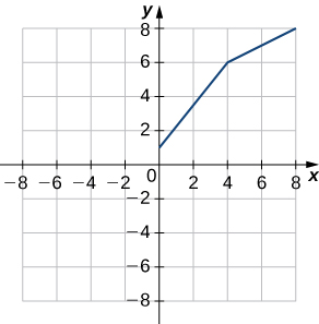
39. Use the following graph to evaluate a. \(f'(1)\) and b. \(f'(6).\)
Solution (click to reveal)
- \(1.25;\) b. \(0.5\)
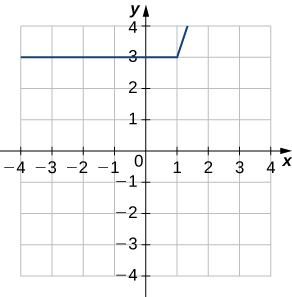
40. Use the following graph to evaluate a. \(f'(-3)\) and b. \(f'(1.5).\)
For the following exercises, use the limit definition of derivative to show that the derivative does not exist at \(x = a\) for each of the given functions.
41. \(f(x) = x^{1\text{/}3},x = 0\)
Solution (click to reveal)
\(\underset{x\rightarrow 0^{-}}{\text{lim}}\frac{x^{1\text{/}3} - 0}{x - 0} = \underset{x\rightarrow 0^{-}}{\text{lim}}\frac{1}{x^{2\text{/}3}} = \infty\)
42. \(f(x) = x^{2\text{/}3},x = 0\)
43. \(f(x) = \left\{ \begin{matrix} {1,x < 1} \\ {x,x \geq 1} \end{matrix} \right.,x = 1\)
Solution (click to reveal)
\(\underset{x\rightarrow 1^{-}}{\text{lim}}\frac{1 - 1}{x - 1} = 0 \neq 1 = \underset{x\rightarrow 1^{+}}{\text{lim}}\frac{x - 1}{x - 1}\)
44. \(f(x) = \frac{|x|}{x},x = 0\)
45. [T] The position in feet of a race car along a straight track after \(t\) seconds is modeled by the function \(s(t) = 8t^{2} - \frac{1}{16}t^{3}.\)
- Find the average velocity of the vehicle over the following time intervals to four decimal places:
- [4, 4.1]
- [4, 4.01]
- [4, 4.001]
- [4, 4.0001]
- Use a. to draw a conclusion about the instantaneous velocity of the vehicle at \(t = 4\) seconds.
Solution (click to reveal)
- \(\text{(i)}\ 61.7244\) ft/s, \(\text{(ii)}\ 61.0725\) ft/s \(\text{(iii)}\ 61.0072\) ft/s \(\text{(iv)}\ 61.0007\) ft/s b. At \(4\) seconds the race car is traveling at a rate/velocity of \(61\) ft/s.
46. [T] The distance in feet that a ball rolls down an incline is modeled by the function \(s(t) = 14t^{2},\) where \(t\) is seconds after the ball begins rolling.
- Find the average velocity of the ball over the following time intervals:
- [5, 5.1]
- [5, 5.01]
- [5, 5.001]
- [5, 5.0001]
- Use the answers from a. to draw a conclusion about the instantaneous velocity of the ball at \(t = 5\) seconds.
47. Two vehicles start out traveling side by side along a straight road. Their position functions, shown in the following graph, are given by \(s = f(t)\) and \(s = g(t),\) where \(s\) is measured in feet and \(t\) is measured in seconds.
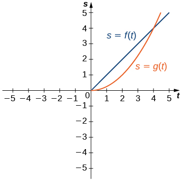
- Which vehicle has traveled farther at \(t = 2\) seconds?
- What is the approximate velocity of each vehicle at \(t = 3\) seconds?
- Which vehicle is traveling faster at \(t = 4\) seconds?
- What is true about the positions of the vehicles at \(t = 4\) seconds?
Solution (click to reveal)
- The vehicle represented by \(f(t),\) because it has traveled \(2\) feet, whereas \(g(t)\) has traveled \(1\) foot. b. The velocity of \(f(t)\) is constant at \(1\) ft/s, while the velocity of \(g(t)\) is approximately \(2\) ft/s. c. The vehicle represented by \(g(t),\) with a velocity of approximately \(4\) ft/s. d. Both have traveled \(4\) feet in \(4\) seconds.
48. [T] The total cost \(C(x),\) in hundreds of dollars, to produce \(x\) thousand jars of mayonnaise is given by \(C(x) = 0.000003x^{3} + 4x + 300.\)
- Calculate the average cost per jar over the following intervals:
- [100, 100.1]
- [100, 100.01]
- [100, 100.001]
- [100, 100.0001]
- Use the answers from a. to estimate the average cost to produce \(100{,}000\) jars of mayonnaise.
49. [T] For the function \(f(x) = x^{3} - 2x^{2} - 11x + 12,\) do the following.
- Use a graphing calculator to graph \(f\) in an appropriate viewing window.
- Use the ZOOM feature on the calculator to approximate the two values of \(x = a\) for which \(m_{\text{tan}} = f'(a) = 0.\)
Solution (click to reveal)
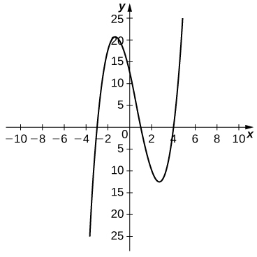
- \(a \approx - 1.361,2.694\)
50. [T] For the function \(f(x) = \frac{x}{1 + x^{2}},\) do the following.
- Use a graphing calculator to graph \(f\) in an appropriate viewing window.
- Use the ZOOM feature on the calculator to approximate the values of \(x = a\) for which \(m_{\text{tan}} = f'(a) = 0.\)
51. Suppose that \(N(x)\) computes the number of gallons of gas used by a vehicle traveling \(x\) miles. Suppose the vehicle gets \(30\) mpg.
- Find a mathematical expression for \(N(x).\)
- What is \(N(100\text{)?}\) Explain the physical meaning.
- What is \(N'(100)?\) Explain the physical meaning.
Solution (click to reveal)
- \(N(x) = \frac{x}{30}\) b. \(\sim 3.3\) gallons. When the vehicle travels \(100\) miles, it has used \(3.3\) gallons of gas. c. \(\frac{1}{30}.\) The rate of gas consumption in gallons per mile that the vehicle is achieving after having traveled \(100\) miles.
52. [T] For the function \(f(x) = x^{4} - 5x^{2} + 4,\) do the following.
- Use a graphing calculator to graph \(f\) in an appropriate viewing window.
- Use the \(\text{nDeriv}\) function, which numerically finds the derivative, on a graphing calculator to estimate \(f'(-2),f'(-0.5),f'(1.7),\) and \(f'(2.718).\)
53. [T] For the function \(f(x) = \frac{x^{2}}{x^{2} + 1},\) do the following.
- Use a graphing calculator to graph \(f\) in an appropriate viewing window.
- Use the \(\text{nDeriv}\) function on a graphing calculator to find \(f'(-4),f'(-2),f'(2),\) and \(f'(4).\)
Solution (click to reveal)
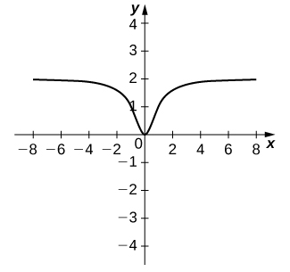
- \(-0.028,-0.16,0.16,0.028\)