1  The Language of Functions

1.1 What Makes a Relationship a Function?

You walk up to a vending machine, press B4, and out drops a bag of pretzels. Press B4 again tomorrow—same pretzels. The machine is reliable: one button, one result. Now imagine a vending machine that dispensed a random item every time you pressed B4. One day pretzels, next day a candy bar, the day after that a granola bar. You’d never trust it. Mathematics demands the same kind of reliability, and the concept that captures it is called a function.

In this section, we’ll make the leap from informal relationships—like “taller people tend to weigh more”—to the precise mathematical idea of a function, where every input determines exactly one output. Along the way, we’ll introduce function notation, explore multiple ways to represent functions, and develop tools for identifying which relationships qualify as functions and which do not.

1.1.1 Relations: Pairing Inputs and Outputs

Before we can say what makes a relationship a function, we need to be clear about what a relationship is in mathematical terms.

NoteDefinition 1.1.1 — Relation

A relation is any set of ordered pairs \((x, y)\). The set of all first coordinates is called the domain, and the set of all second coordinates is called the range.

A relation can be described by a list of ordered pairs, a table, a graph, or a mapping diagram. Figure 1.1.2 shows two relations represented as mapping diagrams. In Relation A, every input maps to exactly one output—this is the kind of reliable, predictable pairing we want. In Relation B, the input \(1\) maps to two different outputs (\(a\) and \(b\)), which means we can’t predict a single result from that input.

Two mapping diagrams side by side. Relation A maps 1 to a, 2 to b, 3 to b, and 4 to c, and is labeled as a function. Relation B maps 1 to both a and b, 2 to b, and 3 to c, and is labeled as not a function.

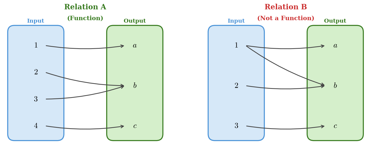
Figure 1.1.2: Two relations shown as mapping diagrams. Relation A is a function; Relation B is not.

The distinction between these two diagrams is the entire point of this section: Relation A is a function, and Relation B is not. Let’s make that idea precise.

1.1.2 Functions and Function Notation

NoteDefinition 1.1.3 — Function

A function is a relation in which each input value corresponds to exactly one output value. If \(f\) is a function and \(x\) is an input, we write \(f(x)\) (read “\(f\) of \(x\)”) for the corresponding output.

The notation \(f(x)\) does not mean “\(f\) times \(x\).” It means “the output of function \(f\) when the input is \(x\).” Think of \(f\) as the name of the machine, \(x\) as what you feed in, and \(f(x)\) as what comes out.

Different letters can name different functions—\(g\), \(h\), \(C\), \(T\)—just as different vending machines dispense different products. The input variable doesn’t have to be \(x\) either; a function tracking temperature over time might be written \(T(t)\), where \(t\) represents hours.

TipExample 1.1.4 — Identifying Functions from Ordered Pairs

Determine whether each relation is a function.

  1. \(\{(1, 3),\; (2, 5),\; (3, 3),\; (4, 7)\}\)
  2. \(\{(2, 1),\; (2, 4),\; (3, 5)\}\)
  3. The table below:
\(x\) \(-1\) \(0\) \(1\) \(2\) \(3\)
\(y\) \(4\) \(2\) \(4\) \(8\) \(14\)

Solution.

  1. Each input (\(1\), \(2\), \(3\), \(4\)) appears exactly once, so each maps to exactly one output. This is a function.

  2. The input \(2\) is paired with both \(1\) and \(4\)—two different outputs for the same input. This is not a function.

  3. Each \(x\)-value appears exactly once in the table, so each input has exactly one output. (Notice that the output \(4\) appears twice, for both \(x = -1\) and \(x = 1\)—that’s perfectly fine. The rule is about inputs, not outputs.) This is a function.

TipExample 1.1.5 — Evaluating a Function from a Formula

Let \(f(x) = 3x^2 - 2x + 5\). Evaluate:

  1. \(f(0)\)
  2. \(f(-2)\)
  3. \(f(a + 1)\)

Solution.

  1. Replace every \(x\) with \(0\): \[f(0) = 3(0)^2 - 2(0) + 5 = 5\]

  2. Replace every \(x\) with \(-2\): \[f(-2) = 3(-2)^2 - 2(-2) + 5 = 3(4) + 4 + 5 = 21\]

  3. Replace every \(x\) with \((a + 1)\): \[f(a + 1) = 3(a + 1)^2 - 2(a + 1) + 5\] Expand: \[= 3(a^2 + 2a + 1) - 2a - 2 + 5 = 3a^2 + 6a + 3 - 2a - 2 + 5 = 3a^2 + 4a + 6\]

TipExample 1.1.6 — Medication Dosage as a Function

A pediatrician uses the formula \(D(w) = 0.15w + 2.5\) to determine the appropriate dosage \(D\) (in mL) of a liquid antibiotic for a child weighing \(w\) pounds.

  1. Find \(D(40)\) and interpret the result.
  2. What is the practical domain of this function?

Solution.

  1. \(D(40) = 0.15(40) + 2.5 = 6 + 2.5 = 8.5\). A child weighing \(40\) pounds should receive \(8.5\) mL of the antibiotic.

  2. The formula works algebraically for any real number, but in context only positive weights make sense. If the formula is designed for children ages 2–12, typical weights might range from about \(25\) to \(100\) pounds. The practical domain is approximately \([25, 100]\).

1.1.3 Representations of Functions

Functions can be described in four main ways: by a formula, a table, a graph, or a verbal description. Each representation has its strengths, and the ability to move between them is one of the most valuable skills in mathematics.

TipExample 1.1.7 — Reading a Function from a Table

A biologist monitors a bacterial colony and records the population \(P\) (in thousands) at various times \(t\) (in hours):

\(t\) (hours) \(0\) \(1\) \(2\) \(3\) \(4\) \(5\)
\(P(t)\) (thousands) \(2.0\) \(3.1\) \(4.8\) \(7.5\) \(11.7\) \(18.2\)
  1. Is \(P\) a function of \(t\)? Explain.
  2. Find \(P(3)\) and interpret the result.
  3. For what value of \(t\) is \(P(t) = 4.8\)?

Solution.

  1. Yes. Each time value \(t\) corresponds to exactly one population value \(P(t)\), so \(P\) is a function of \(t\).

  2. From the table, \(P(3) = 7.5\). After \(3\) hours, the colony contains approximately \(7{,}500\) bacteria.

  3. From the table, \(P(2) = 4.8\), so \(t = 2\) hours.

When a function is represented as a graph, we read it by looking up input values on the horizontal axis and finding the corresponding output on the curve. Figure 1.1.8 shows the temperature in a city over a \(24\)-hour period.

Graph of temperature in degrees Fahrenheit over 24 hours, with a low of 48 degrees at 2 a.m. and a high of 82 degrees at 4 p.m.

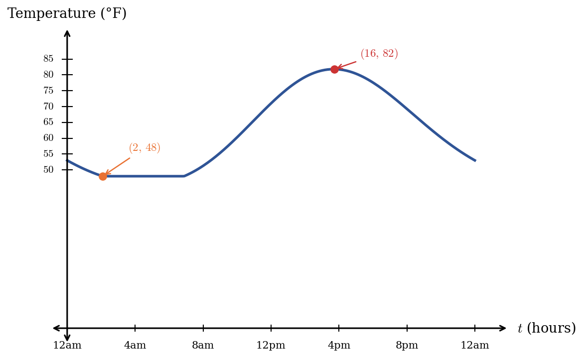
Figure 1.1.8: Outdoor temperature (°F) over a \(24\)-hour period. The low occurs around \(t = 2\) (2:00 AM) and the high around \(t = 16\) (4:00 PM).

TipExample 1.1.9 — Reading Function Values from a Graph

Use Figure 1.1.8 to answer each question.

  1. What is the temperature at 8:00 AM (\(t = 8\))?
  2. At approximately what time(s) is the temperature \(70\)°F?
  3. What are the domain and range of this function?

Solution.

  1. Locate \(t = 8\) on the horizontal axis and read across to the curve: \(T(8) \approx 58\)°F.

  2. Draw a horizontal line at \(T = 70\). It crosses the curve at approximately \(t \approx 10\) (10:00 AM) and again at \(t \approx 21\) (9:00 PM).

  3. The graph spans from \(t = 0\) to \(t = 24\), so the domain is \([0, 24]\). The temperature ranges from a low of about \(48\)°F to a high of about \(82\)°F, so the range is approximately \([48, 82]\).

1.1.4 The Vertical Line Test

When a relation is given as a graph, there is a quick visual test for whether it is a function.

NoteDefinition 1.1.10 — The Vertical Line Test

A curve in the \(xy\)-plane is the graph of a function of \(x\) if and only if no vertical line intersects the curve more than once.

The logic is straightforward: a vertical line through \(x = a\) hits the graph at every point whose input is \(a\). If the line hits the curve twice, then the input \(a\) produces two different outputs—and that violates the definition of a function.

Figure 1.1.11 shows two curves. On the left, every vertical line crosses the cubic curve at most once, so it represents a function. On the right, the vertical line crosses the circle at two points, confirming that the circle is not the graph of a function.

Two graphs side by side. On the left, a cubic curve passes the vertical line test with one intersection point shown. On the right, a circle fails the vertical line test with two intersection points shown.

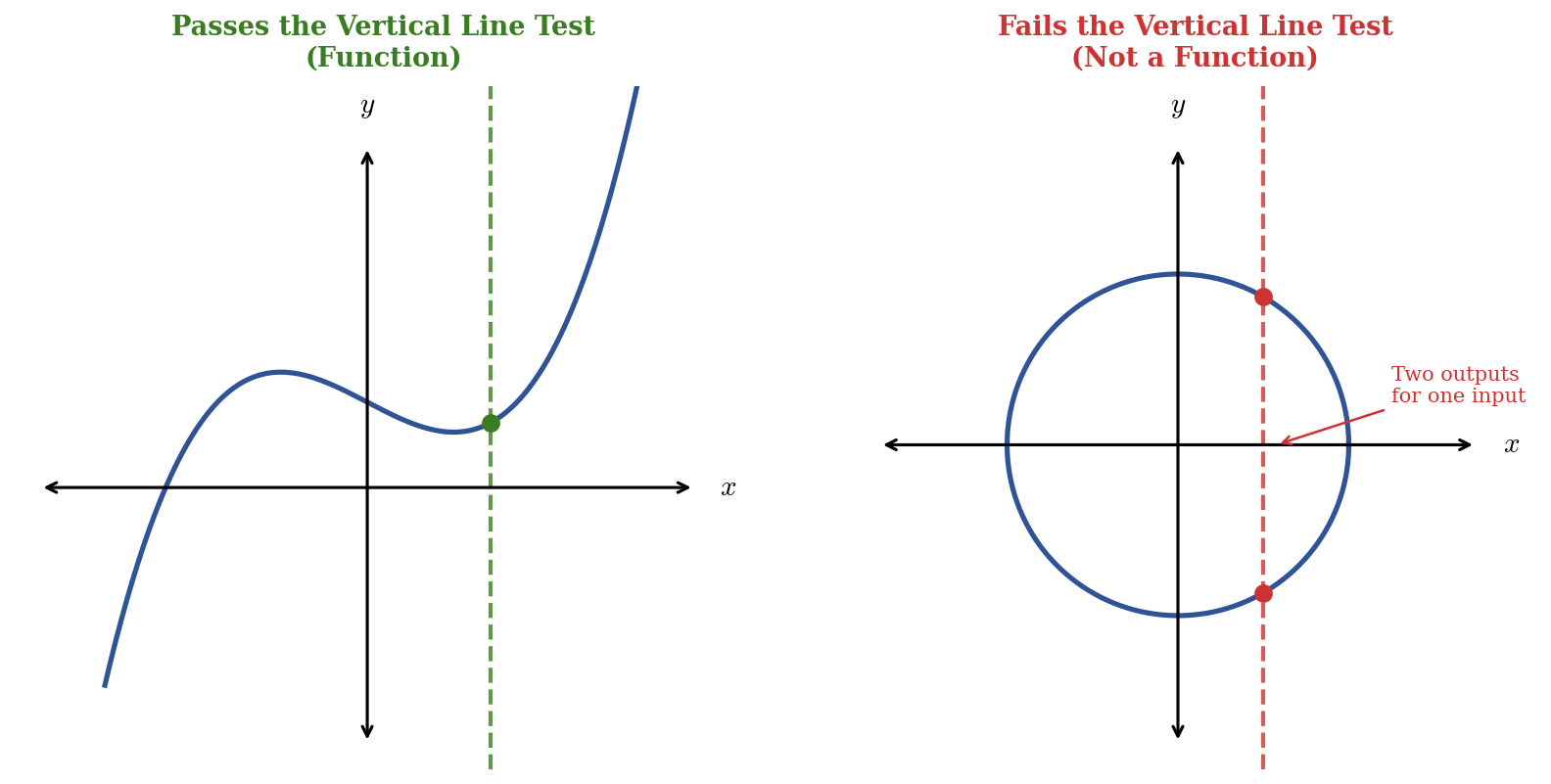
Figure 1.1.11: The vertical line test. Left: a function (each vertical line hits the curve once). Right: not a function (a vertical line hits the circle twice).

TipExample 1.1.12 — Applying the Vertical Line Test

Determine whether each equation defines \(y\) as a function of \(x\):

  1. \(y = x^2 - 4\)
  2. \(x = y^2\)
  3. \(x^2 + y^2 = 9\)

Solution.

  1. For any value of \(x\), the expression \(x^2 - 4\) produces exactly one value of \(y\). Equivalently, the graph is a parabola opening upward, which passes the vertical line test. This is a function.

  2. Solving for \(y\) gives \(y = \pm\sqrt{x}\). For any positive \(x\), there are two corresponding \(y\)-values (one positive, one negative). For instance, when \(x = 4\), \(y = 2\) or \(y = -2\). This is not a function.

  3. This is the equation of a circle with radius \(3\). Solving for \(y\) gives \(y = \pm\sqrt{9 - x^2}\), which again yields two outputs for most inputs. This is not a function.

1.1.5 Domain and Range

NoteDefinition 1.1.13 — Domain and Range

The domain of a function is the set of all allowable input values. The range is the set of all output values that the function actually produces.

When a function is defined by a formula with no real-world context, the domain consists of all real numbers for which the formula produces a real output. Two common restrictions arise:

  • Division by zero is undefined: Exclude input values that make a denominator equal to zero.
  • Square roots of negative numbers are not real: Exclude input values that make the expression under an even root negative.

We express domains using interval notation: \((a, b)\) means all numbers strictly between \(a\) and \(b\); \([a, b]\) includes the endpoints; and \((-\infty, \infty)\) means all real numbers. A union symbol \(\cup\) joins disconnected intervals: for example, \((-\infty, 2) \cup (2, \infty)\) means all real numbers except \(2\).

TipExample 1.1.14 — Finding Domains from Formulas

Find the domain of each function.

  1. \(f(x) = \dfrac{1}{x - 3}\)
  2. \(g(x) = \sqrt{x + 4}\)
  3. \(h(x) = x^2 - 6x + 1\)

Solution.

  1. The denominator is zero when \(x = 3\), so we exclude that value. The domain is \((-\infty, 3) \cup (3, \infty)\).

  2. The expression under the square root must be non-negative: \(x + 4 \geq 0\), so \(x \geq -4\). The domain is \([-4, \infty)\).

  3. A polynomial is defined for all real numbers—there is no division and no even root. The domain is \((-\infty, \infty)\).

TipExample 1.1.15 — Domain of an Average Cost Function

A small business finds that the average cost (in dollars) of producing \(x\) units of a product is given by

\[C(x) = \frac{500 + 8x}{x}\]

Find the domain of \(C\).

Solution. The function is undefined when the denominator equals zero: \(x = 0\). In mathematical terms, the domain is \((-\infty, 0) \cup (0, \infty)\). In the business context, producing a negative number of units makes no sense, so the practical domain is \((0, \infty)\)—that is, any positive number of units.

When working from a graph, the domain is the set of \(x\)-values covered by the curve, and the range is the set of \(y\)-values.

TipExample 1.1.16 — Domain and Range from a Graph

A patient undergoes a cardiac stress test. Figure 1.1.17 shows the patient’s heart rate \(H(t)\) (in beats per minute) as a function of time \(t\) (in minutes).

Graph of heart rate in beats per minute over 20 minutes during a stress test. Heart rate begins at 70 bpm, rises to a peak of 172 bpm at 13 minutes, then declines to 94 bpm at 20 minutes.

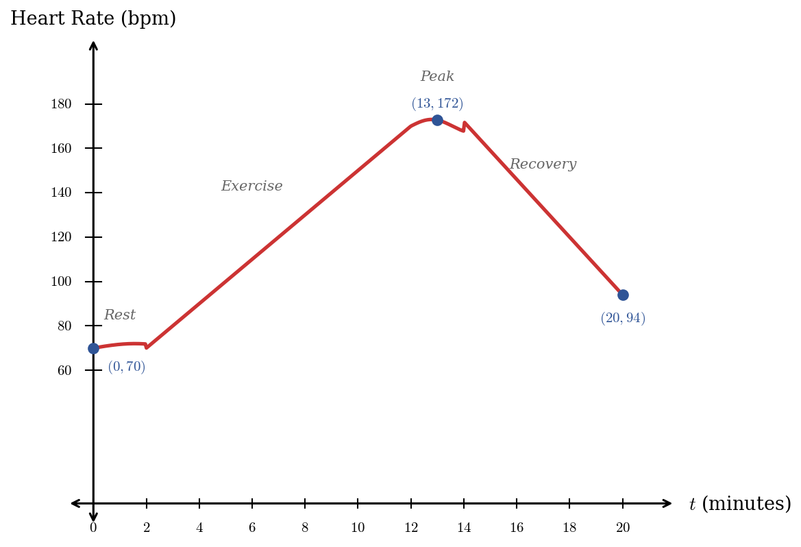
Figure 1.1.17: Heart rate during a cardiac stress test.

  1. What are the domain and range of \(H\)?
  2. Interpret \(H(13) = 172\) in context.
  3. During which time interval is the heart rate increasing?

Solution.

  1. The graph spans from \(t = 0\) to \(t = 20\), so the domain is \([0, 20]\). The heart rate ranges from a resting value of about \(70\) bpm to a peak of about \(172\) bpm, so the range is approximately \([70, 172]\).

  2. After \(13\) minutes of the stress test, the patient’s heart rate reached its peak of \(172\) beats per minute.

  3. The heart rate is increasing from \(t = 0\) to approximately \(t = 13\), during the rest, exercise, and peak phases.

1.1.6 Piecewise-Defined Functions

Sometimes a single formula isn’t enough to describe how a function behaves across its entire domain. When different rules apply to different input ranges, we use a piecewise-defined function.

NoteDefinition 1.1.18 — Piecewise-Defined Function

A piecewise-defined function is a function described by two or more formulas, each applying to a different part of the domain.

The key skill with piecewise functions is choosing the right formula: look at the input value, determine which piece of the domain it falls into, then use the corresponding rule.

TipExample 1.1.19 — Evaluating a Piecewise Function

Let

\[ f(x) = \begin{cases} x^2 & \text{if } x < 1 \\ 3x - 1 & \text{if } x \geq 1 \end{cases} \]

Evaluate \(f(-2)\), \(f(1)\), and \(f(4)\).

Solution.

For \(f(-2)\): Since \(-2 < 1\), use the first rule: \(f(-2) = (-2)^2 = 4\).

For \(f(1)\): Since \(1 \geq 1\), use the second rule: \(f(1) = 3(1) - 1 = 2\).

For \(f(4)\): Since \(4 \geq 1\), use the second rule: \(f(4) = 3(4) - 1 = 11\).

The graph of this function, shown in Figure 1.1.20, consists of a parabola to the left of \(x = 1\) and a line from \(x = 1\) onward. The open circle at \((1, 1)\) indicates that the parabola does not include that endpoint, while the closed circle at \((1, 2)\) shows that the linear piece does.

Graph of a piecewise function. For x less than 1, the graph is a parabola y equals x squared with an open circle at the point 1 comma 1. For x greater than or equal to 1, the graph is a line y equals 3x minus 1 with a closed circle at the point 1 comma 2.

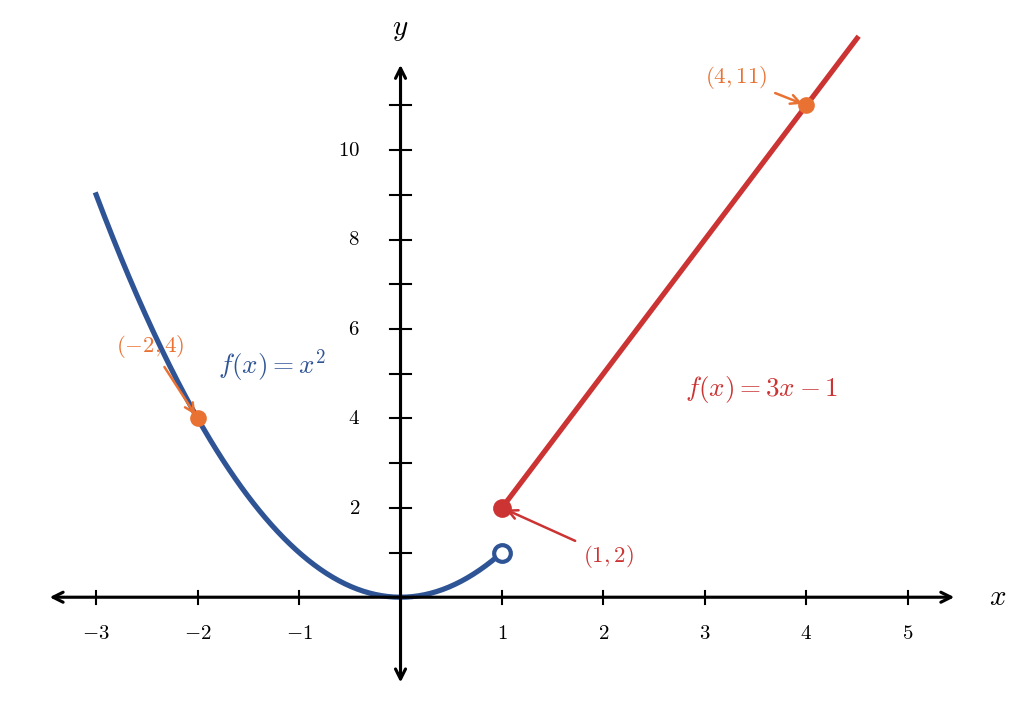
Figure 1.1.20: Graph of \(f(x) = x^2\) for \(x < 1\) and \(f(x) = 3x - 1\) for \(x \geq 1\).

TipExample 1.1.21 — A Cell Phone Data Plan

A wireless carrier offers a data plan that charges a flat fee of $45 per month for up to \(5\) GB of data. Each additional gigabyte beyond \(5\) GB costs $10. The monthly cost \(C(d)\) (in dollars) as a function of data usage \(d\) (in GB) is:

\[ C(d) = \begin{cases} 45 & \text{if } 0 \leq d \leq 5 \\ 45 + 10(d - 5) & \text{if } d > 5 \end{cases} \]

  1. Find \(C(3)\) and \(C(8)\) and interpret each.
  2. A customer’s bill is $75. How many gigabytes did they use?
  3. What are the domain and range of \(C\)?

Solution.

  1. Since \(3 \leq 5\), we use the first rule: \(C(3) = 45\). A customer using \(3\) GB pays $45. Since \(8 > 5\), we use the second rule: \(C(8) = 45 + 10(8 - 5) = 45 + 30 = 75\). A customer using \(8\) GB pays $75.

  2. Since the bill exceeds $45, the customer used more than \(5\) GB. Setting the second rule equal to \(75\): \[45 + 10(d - 5) = 75 \quad \Longrightarrow \quad 10(d - 5) = 30 \quad \Longrightarrow \quad d = 8 \text{ GB}\]

  3. The input \(d\) represents data usage, so \(d \geq 0\) and the domain is \([0, \infty)\). The minimum cost is $45 (for \(0\)\(5\) GB) and there is no upper limit, so the range is \([45, \infty)\).

Graph of a piecewise function showing monthly cost in dollars versus data usage in gigabytes. The cost is flat at 45 dollars from 0 to 5 GB, then increases linearly at 10 dollars per GB beyond 5 GB.

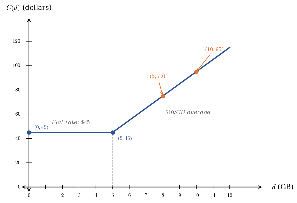
Figure 1.1.22: Monthly cost of the data plan as a function of data usage.

1.1.7 Summary

  • A relation is any set of ordered pairs. A function is a relation in which each input has exactly one output.
  • We write \(f(x)\) for the output of function \(f\) at input \(x\). This is called function notation.
  • Functions can be represented by formulas, tables, graphs, or verbal descriptions.
  • The vertical line test determines whether a graph represents a function: if any vertical line crosses the graph more than once, it is not a function.
  • The domain is the set of all allowable inputs; the range is the set of all resulting outputs.
  • When finding the domain from a formula, exclude values that cause division by zero or square roots of negative numbers.
  • A piecewise-defined function uses different formulas for different parts of the domain.

1.2 Measuring Change: Secant Lines and the Difference Quotient

Your car’s speedometer reads \(65\) mph, but you’ve been stuck in stop-and-go traffic for the last hour and only covered \(30\) miles. The speedometer measures your speed right now; the \(30\)-miles-in-one-hour figure measures your average speed. This distinction—between instantaneous and average rates of change—is one of the most important ideas in mathematics. In this section, we develop tools for measuring average rates of change: the secant line and the difference quotient.

Every time you compute “how much something changed divided by how long it took,” you’re computing an average rate of change. Gas mileage, grade point averages, even batting averages—all of these are ratios of change. We’ll make this idea precise using function notation and build the algebraic skills you’ll need when these ideas resurface in calculus.

1.2.1 Secant Lines and Average Rate of Change

NoteDefinition 1.2.1 — Secant Line

A secant line to the graph of a function \(f\) is a line that intersects the curve at two distinct points.

Given a function \(f\) and two points on its graph, \((a, f(a))\) and \((b, f(b))\), the secant line is the straight line connecting these points. The slope of this secant line measures how much the output changes, on average, as the input moves from \(a\) to \(b\).

NoteDefinition 1.2.2 — Average Rate of Change

The average rate of change of a function \(f\) over the interval \([a, b]\) is the slope of the secant line connecting \((a, f(a))\) and \((b, f(b))\):

\[ \text{Average Rate of Change} = \frac{f(b) - f(a)}{b - a} \]

Figure 1.2.3 illustrates this relationship. The horizontal distance \(b - a\) represents the change in input, while the vertical distance \(f(b) - f(a)\) represents the change in output. Their ratio gives the slope of the secant line.

Graph showing a curve y equals f of x with two points labeled a comma f of a and b comma f of b connected by a secant line. The horizontal distance b minus a and vertical distance f of b minus f of a are marked.

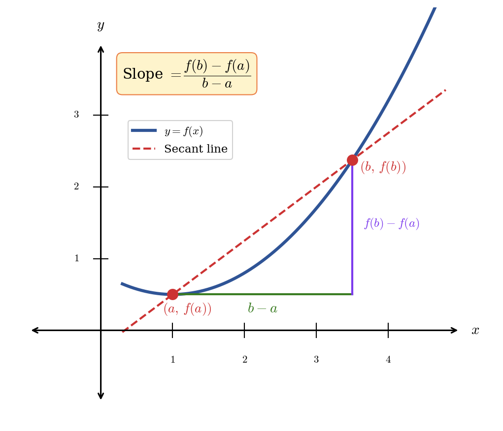
Figure 1.2.3: The secant line connecting \((a, f(a))\) and \((b, f(b))\) on the graph of \(f\).

The average rate of change tells us how the function behaves on average between two points—but it doesn’t tell us what’s happening at any specific instant. Think of driving \(150\) miles in \(3\) hours: your average speed was \(50\) mph, even if you were sometimes going \(70\) mph and sometimes crawling through a school zone at \(10\).

1.2.2 The Difference Quotient

When studying rates of change, we often want to examine what happens near a particular input value \(x\). Instead of using two separate variables \(a\) and \(b\), we use \(x\) for our starting point and \(x + h\) for a nearby point, where \(h\) represents a small horizontal shift.

With this notation, \(b - a\) becomes \((x + h) - x = h\), and the average rate of change formula transforms into the difference quotient.

NoteDefinition 1.2.4 — The Difference Quotient

For a function \(f(x)\), the difference quotient is:

\[ \frac{f(x + h) - f(x)}{h}, \quad h \neq 0 \]

Let’s break down what this expression means:

  • \(f(x)\) is the output of our function at some starting point \(x\)
  • \(f(x + h)\) is the output at a nearby point, where \(h\) represents a small horizontal shift
  • The numerator \(f(x + h) - f(x)\) measures how much the output changed
  • Dividing by \(h\) tells us the change in output per unit of input

Geometrically, the difference quotient gives the slope of the secant line connecting the points \((x, f(x))\) and \((x + h, f(x + h))\) on the graph of \(f\), as shown in Figure 1.2.5.

Graph showing a curve y equals f of x with two points labeled x comma f of x and x plus h comma f of x plus h connected by a secant line. The horizontal distance h and vertical distance f of x plus h minus f of x are marked.

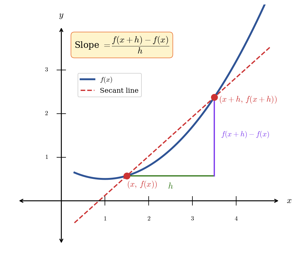
Figure 1.2.5: The difference quotient as the slope of a secant line through \((x, f(x))\) and \((x + h, f(x + h))\).

Why Does This Matter?

The difference quotient appears throughout science and engineering:

  • Physics: Average velocity is the difference quotient of position with respect to time.
  • Economics: Marginal cost approximations use difference quotients to estimate how costs change with production levels.
  • Biology: Population growth rates are computed as difference quotients of population size over time.

In calculus, you’ll take the limit of the difference quotient as \(h\) approaches zero, which gives the instantaneous rate of change—the derivative. Mastering the algebraic techniques in this section will prepare you for that transition.

1.2.3 Computing Difference Quotients

Computing a difference quotient is a three-step process: find \(f(x + h)\), compute \(f(x + h) - f(x)\), and divide by \(h\) and simplify. The algebra varies depending on the type of function. Let’s work through the main cases.

TipExample 1.2.6 — A Quadratic Function

Compute the difference quotient for \(f(x) = 2x^2 + x - 5\).

Solution.

Step 1: Find \(f(x + h)\) by replacing every \(x\) with \((x + h)\):

\[ f(x + h) = 2(x + h)^2 + (x + h) - 5 \]

Expand \((x + h)^2 = x^2 + 2xh + h^2\):

\[ f(x + h) = 2(x^2 + 2xh + h^2) + x + h - 5 = 2x^2 + 4xh + 2h^2 + x + h - 5 \]

Step 2: Compute \(f(x + h) - f(x)\):

\[ f(x + h) - f(x) = (2x^2 + 4xh + 2h^2 + x + h - 5) - (2x^2 + x - 5) = 4xh + 2h^2 + h \]

Step 3: Divide by \(h\):

\[ \frac{f(x + h) - f(x)}{h} = \frac{4xh + 2h^2 + h}{h} = \frac{h(4x + 2h + 1)}{h} = 4x + 2h + 1 \]

Result: The difference quotient is \(4x + 2h + 1\).

Figure 1.2.7 illustrates this example with specific values \(x = 1\) and \(h = 1\), giving a secant line with slope \(4(1) + 2(1) + 1 = 7\).

Graph of f of x equals 2x squared plus x minus 5 showing points 1 comma negative 2 and 2 comma 5 connected by a secant line with slope 7.

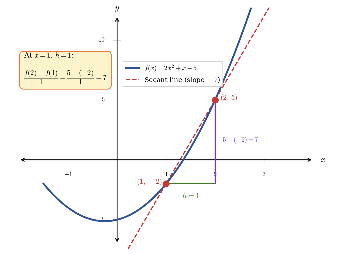
Figure 1.2.7: The secant line for \(f(x) = 2x^2 + x - 5\) with \(x = 1\) and \(h = 1\), showing slope \(= 7\).

Notice that as \(h\) gets smaller, this expression approaches \(4x + 1\)—which, as you’ll learn in calculus, is the derivative of \(f(x) = 2x^2 + x - 5\).

TipExample 1.2.8 — A Rational Function

Compute the difference quotient for \(f(x) = \frac{1}{x}\).

Solution.

Step 1: Write \(f(x + h)\):

\[ f(x + h) = \frac{1}{x + h} \]

Step 2: Compute \(f(x + h) - f(x)\):

\[ f(x + h) - f(x) = \frac{1}{x + h} - \frac{1}{x} \]

To subtract these fractions, find a common denominator:

\[ = \frac{x}{x(x + h)} - \frac{x + h}{x(x + h)} = \frac{x - (x + h)}{x(x + h)} = \frac{-h}{x(x + h)} \]

Step 3: Divide by \(h\):

\[ \frac{f(x + h) - f(x)}{h} = \frac{-h}{x(x + h)} \cdot \frac{1}{h} = \frac{-1}{x(x + h)} \]

Result: The difference quotient is \(\displaystyle\frac{-1}{x(x + h)}\).

The negative sign tells us that \(f(x) = \frac{1}{x}\) is decreasing for positive \(x\)—as \(x\) increases, \(\frac{1}{x}\) decreases.

TipExample 1.2.9 — A Square Root Function

Compute the difference quotient for \(f(x) = \sqrt{x}\).

Solution.

Step 1: Write \(f(x + h)\):

\[ f(x + h) = \sqrt{x + h} \]

Step 2: Compute \(f(x + h) - f(x)\):

\[ f(x + h) - f(x) = \sqrt{x + h} - \sqrt{x} \]

Step 3: Divide by \(h\):

\[ \frac{f(x + h) - f(x)}{h} = \frac{\sqrt{x + h} - \sqrt{x}}{h} \]

This expression doesn’t simplify easily in its current form. To simplify, we rationalize the numerator by multiplying by the conjugate:

\[ = \frac{\sqrt{x + h} - \sqrt{x}}{h} \cdot \frac{\sqrt{x + h} + \sqrt{x}}{\sqrt{x + h} + \sqrt{x}} \]

The numerator becomes a difference of squares:

\[ = \frac{(x + h) - x}{h\left(\sqrt{x + h} + \sqrt{x}\right)} = \frac{h}{h\left(\sqrt{x + h} + \sqrt{x}\right)} = \frac{1}{\sqrt{x + h} + \sqrt{x}} \]

Result: The difference quotient is \(\displaystyle\frac{1}{\sqrt{x + h} + \sqrt{x}}\).

This example illustrates an important algebraic technique—rationalizing—that you’ll use frequently when working with radical expressions.

1.2.4 Summary

  • Secant line: A line that intersects the graph of a function at two distinct points.
  • Average rate of change of \(f\) over \([a, b]\): \(\displaystyle\frac{f(b) - f(a)}{b - a}\)
  • Difference quotient: \(\displaystyle\frac{f(x + h) - f(x)}{h}\) measures the average rate of change near a point \(x\).
  • Computing difference quotients requires careful algebra:
    • For polynomial functions, expand, subtract, and factor out \(h\).
    • For rational functions, find common denominators before simplifying.
    • For radical functions, rationalize the numerator using conjugates.

These techniques will serve you well not only in this course but as essential preparation for calculus.

1.3 Shifting, Stretching, Reflecting: Transformations of Functions

Open a photo on your phone and play with the editing tools. Slide the brightness up, and the whole image gets lighter — the content doesn’t change, just how bright it appears. Flip the photo horizontally, and your selfie becomes a mirror image. Crop and reposition, and the same scene sits in a different spot on the screen. In every case, you’re transforming the image without changing what’s actually in it.

Functions work the same way. Starting from a small collection of basic shapes — parabolas, square roots, absolute values — we can shift them up, down, left, or right; stretch or compress them; and flip them across an axis. These transformations let us build an enormous variety of functions from just a handful of building blocks. Mastering them means you can look at a complicated formula like \(g(x) = -2|x - 3| + 4\) and immediately picture its graph, without plotting a single point.

1.3.1 Parent Functions

Every family of functions has a simplest member, called the parent function. These are the building blocks we’ll transform throughout this section.

NoteDefinition 1.3.1 — Parent Function

A parent function is the simplest function in a family of functions that share the same basic shape. All other members of the family can be obtained by applying transformations to the parent.

Figure 1.3.2 displays six parent functions you’ll encounter repeatedly in this course. Becoming familiar with their shapes is essential — when you see a transformed version, you’ll want to recognize which parent it came from.

Six parent functions displayed in a grid: f of x equals x (linear), f of x equals x squared (quadratic), f of x equals x cubed (cubic), f of x equals square root of x, f of x equals absolute value of x, and f of x equals 1 over x (reciprocal).

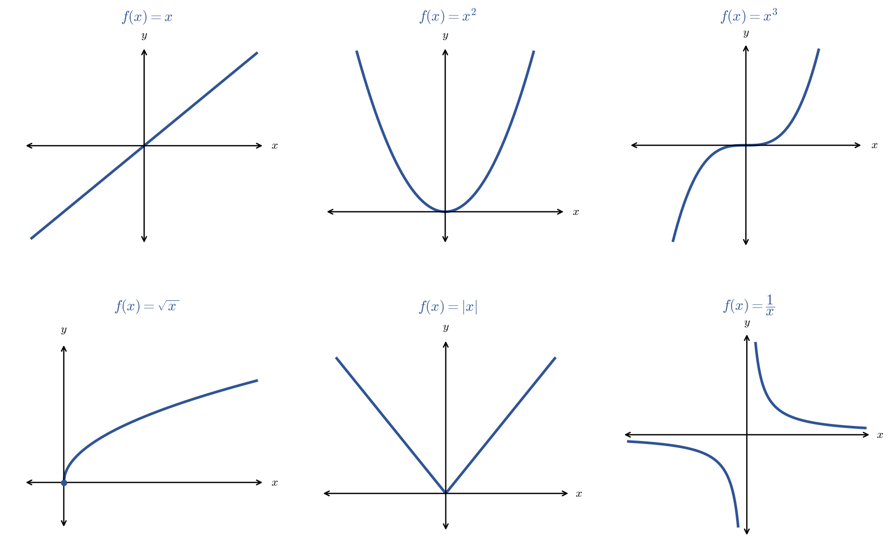
Figure 1.3.2: The six parent functions: identity, quadratic, cubic, square root, absolute value, and reciprocal.

TipExample 1.3.3 — Identifying Parent Functions

Identify the parent function for each:

  1. \(g(x) = 3x^2 - 5\)
  2. \(h(x) = \sqrt{x + 7} - 1\)
  3. \(k(x) = -\dfrac{4}{x}\)

Solution.

  1. The dominant term is \(x^2\), so the parent is \(f(x) = x^2\). The graph is a parabola that has been vertically stretched and shifted down.

  2. The key operation is the square root, so the parent is \(f(x) = \sqrt{x}\). The graph is a square root curve that has been shifted left and down.

  3. The key structure is division by \(x\), so the parent is \(f(x) = \dfrac{1}{x}\). The graph is a reciprocal function that has been vertically stretched and reflected.

1.3.2 Vertical and Horizontal Shifts

The simplest transformations move a graph without changing its shape.

NoteDefinition 1.3.4 — Vertical and Horizontal Shifts

Let \(f\) be a function and let \(k\) and \(h\) be positive constants.

Vertical shifts:

  • \(g(x) = f(x) + k\) shifts the graph of \(f\) up by \(k\) units.
  • \(g(x) = f(x) - k\) shifts the graph of \(f\) down by \(k\) units.

Horizontal shifts:

  • \(g(x) = f(x - h)\) shifts the graph of \(f\) right by \(h\) units.
  • \(g(x) = f(x + h)\) shifts the graph of \(f\) left by \(h\) units.

Vertical shifts are intuitive: adding a constant to every output moves every point on the graph up or down by the same amount. Figure 1.3.5 shows \(f(x) = x^2\) alongside \(g(x) = x^2 + 3\) (shifted up \(3\)) and \(h(x) = x^2 - 2\) (shifted down \(2\)).

Three parabolas on the same axes. The parent f of x equals x squared in blue, g of x equals x squared plus 3 shifted up in green, and h of x equals x squared minus 2 shifted down in red.

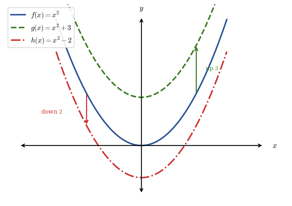
Figure 1.3.5: Vertical shifts of \(f(x) = x^2\).

Horizontal shifts are trickier. Notice the opposite sign pattern: \(f(x - 2)\) shifts the graph right (not left), and \(f(x + 3)\) shifts it left (not right). Why? To get the same output that \(f\) originally produced at \(x = 0\), you now need to input \(x = 2\) in \(f(x - 2)\), because \(f(2 - 2) = f(0)\). Every point on the graph must move \(2\) units to the right to compensate. Figure 1.3.6 illustrates this with \(g(x) = (x - 2)^2\) and \(h(x) = (x + 3)^2\).

Three parabolas showing horizontal shifts. The parent f of x equals x squared centered at the origin, g of x equals open parenthesis x minus 2 close parenthesis squared shifted right 2, and h of x equals open parenthesis x plus 3 close parenthesis squared shifted left 3.

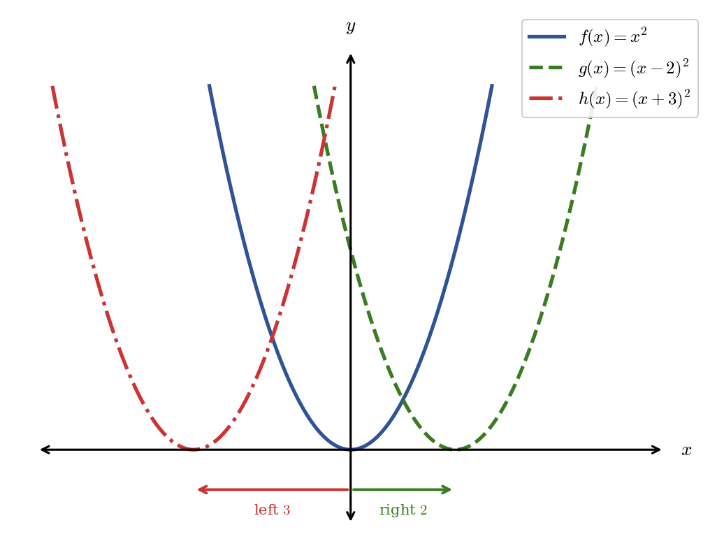
Figure 1.3.6: Horizontal shifts of \(f(x) = x^2\).

TipExample 1.3.7 — Describing Shifts

Without graphing, describe the transformation and identify the parent function.

  1. \(g(x) = \sqrt{x - 4} + 2\)
  2. \(h(x) = (x + 1)^3 - 6\)
  3. \(k(x) = |x| - 3\)

Solution.

  1. The parent is \(f(x) = \sqrt{x}\). Writing \(g(x) = f(x - 4) + 2\), we see this is a shift right \(4\) and up \(2\). The starting point moves from \((0, 0)\) to \((4, 2)\).

  2. The parent is \(f(x) = x^3\). Writing \(h(x) = f(x + 1) - 6\), this is a shift left \(1\) and down \(6\). The inflection point moves from \((0, 0)\) to \((-1, -6)\).

  3. The parent is \(f(x) = |x|\). This is simply a shift down \(3\). The vertex moves from \((0, 0)\) to \((0, -3)\).

TipExample 1.3.8 — Shifting a Temperature Model

An environmental scientist models the daily temperature in City A as \(T_A(t) = 15 + 12\sin\!\left(\frac{\pi}{12}(t - 8)\right)\) where \(t\) is hours after midnight and temperature is in degrees Celsius. City B, \(200\) miles to the north, experiences the same daily pattern but \(3\)°C cooler and with the peak occurring \(2\) hours later.

Write a function \(T_B(t)\) for City B’s temperature.

Solution. The phrase “same pattern but \(3\)°C cooler” means we shift the output down \(3\): subtract \(3\). The phrase “\(2\) hours later” means the same temperatures occur \(2\) hours later in the day, which is a shift right \(2\): replace \(t\) with \((t - 2)\).

\[T_B(t) = T_A(t - 2) - 3 = 15 + 12\sin\!\left(\frac{\pi}{12}((t-2) - 8)\right) - 3 = 12 + 12\sin\!\left(\frac{\pi}{12}(t - 10)\right)\]

1.3.3 Reflections

A reflection flips a graph across an axis, producing a mirror image.

NoteDefinition 1.3.9 — Reflections

Let \(f\) be a function.

  • \(g(x) = -f(x)\) reflects the graph of \(f\) across the \(x\)-axis. Every \(y\)-coordinate is negated.
  • \(g(x) = f(-x)\) reflects the graph of \(f\) across the \(y\)-axis. Every \(x\)-coordinate is negated.

Figure 1.3.10 shows both reflections applied to \(f(x) = \sqrt{x}\). The \(x\)-axis reflection \(g(x) = -\sqrt{x}\) flips the curve downward, while the \(y\)-axis reflection \(h(x) = \sqrt{-x}\) flips it to the left.

Three curves on the same axes. The parent f of x equals square root of x in the first quadrant, g of x equals negative square root of x reflected below the x-axis, and h of x equals square root of negative x reflected into the second quadrant.

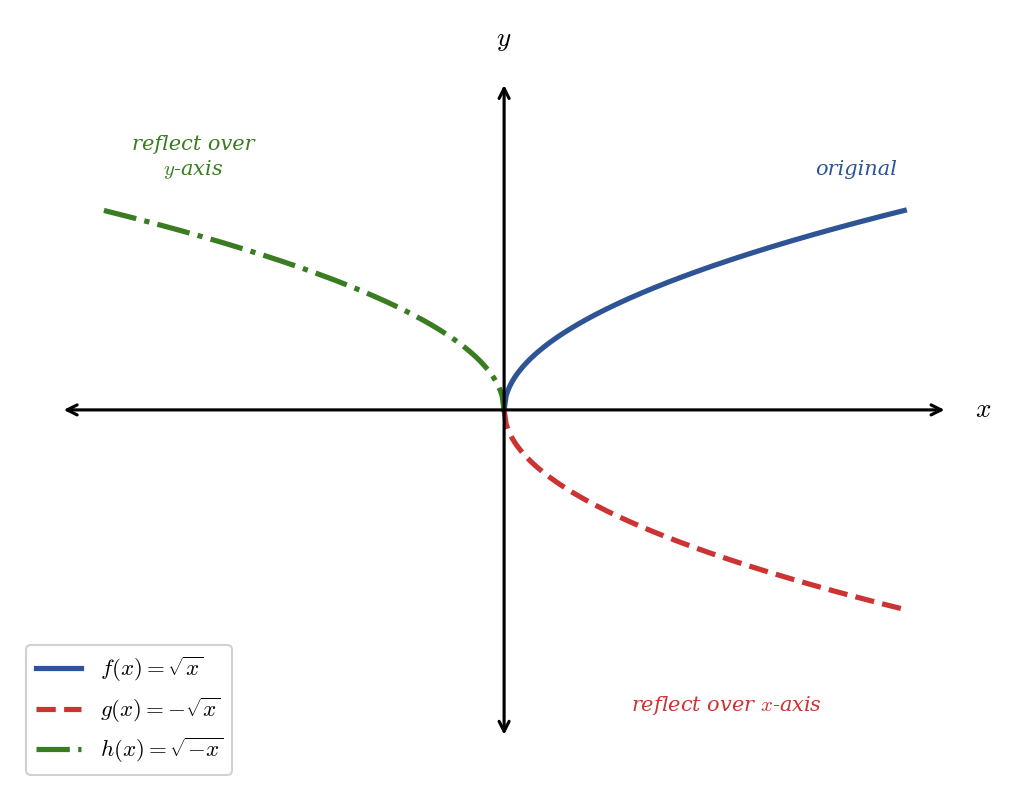
Figure 1.3.10: Reflections of \(f(x) = \sqrt{x}\) across the \(x\)-axis and \(y\)-axis.

TipExample 1.3.11 — Identifying Reflections

Starting from \(f(x) = x^2\), describe how each function is related to \(f\).

  1. \(g(x) = -x^2\)
  2. \(h(x) = (-x)^2\)

Solution.

  1. \(g(x) = -f(x)\): this is a reflection across the \(x\)-axis. The parabola opens downward instead of upward.

  2. \(h(x) = f(-x) = (-x)^2 = x^2 = f(x)\). Reflecting \(x^2\) across the \(y\)-axis produces the same graph! This makes sense because \(x^2\) is symmetric about the \(y\)-axis. (We’ll revisit this idea in the section on even and odd functions.)

1.3.4 Vertical and Horizontal Stretches and Compressions

Stretches and compressions change the scale of a graph — making it taller, shorter, wider, or narrower — without changing its basic shape.

NoteDefinition 1.3.12 — Vertical Stretch and Compression

Let \(f\) be a function and \(a > 0\) a constant.

  • If \(a > 1\), then \(g(x) = a \cdot f(x)\) stretches the graph of \(f\) vertically by a factor of \(a\). The graph becomes taller.
  • If \(0 < a < 1\), then \(g(x) = a \cdot f(x)\) compresses the graph of \(f\) vertically by a factor of \(a\). The graph becomes shorter.

Figure 1.3.14 compares \(f(x) = x^2\) with \(g(x) = 2x^2\) (stretched — steeper, narrower appearance) and \(h(x) = \frac{1}{2}x^2\) (compressed — flatter, wider appearance).

Three parabolas. The parent x squared in blue, 2 x squared stretched vertically in green, and one-half x squared compressed vertically in red.

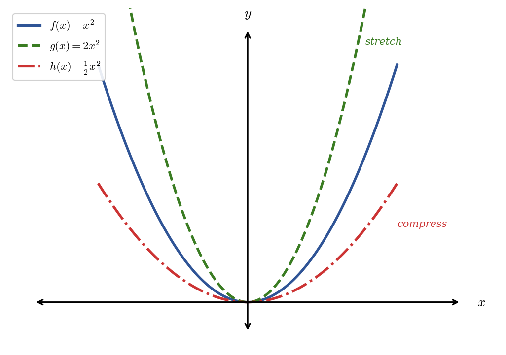
Figure 1.3.14: Vertical stretch and compression of \(f(x) = x^2\).

NoteDefinition 1.3.13 — Horizontal Stretch and Compression

Let \(f\) be a function and \(b > 0\) a constant.

  • If \(b > 1\), then \(g(x) = f(bx)\) compresses the graph of \(f\) horizontally by a factor of \(\frac{1}{b}\). The graph becomes narrower.
  • If \(0 < b < 1\), then \(g(x) = f(bx)\) stretches the graph of \(f\) horizontally by a factor of \(\frac{1}{b}\). The graph becomes wider.

Just as with horizontal shifts, the horizontal direction is counterintuitive: multiplying the input by \(2\) makes the graph narrower (not wider), because each output value is reached at half the original \(x\)-value. Figure 1.3.15 illustrates this.

Three parabolas showing horizontal scaling. The parent x squared in blue, open parenthesis 2x close parenthesis squared compressed horizontally in green, and open parenthesis one-half x close parenthesis squared stretched horizontally in red.

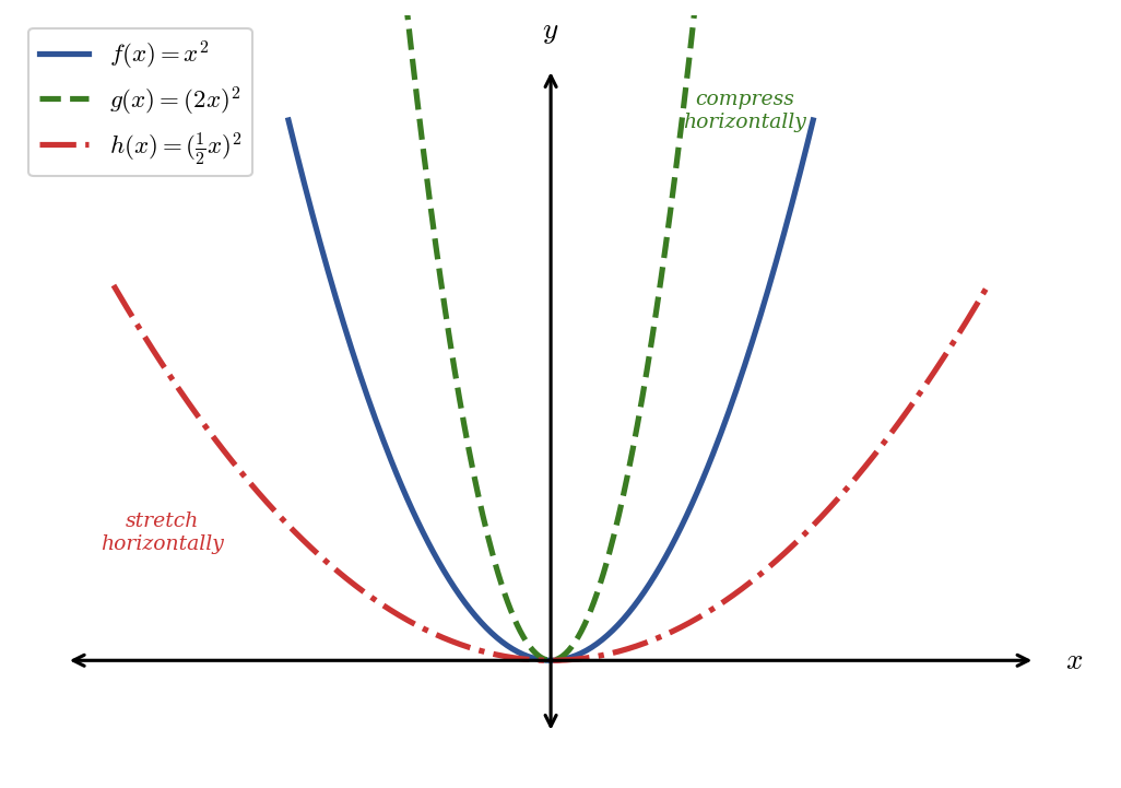
Figure 1.3.15: Horizontal stretch and compression of \(f(x) = x^2\).

TipExample 1.3.16 — Describing Stretches and Compressions

Starting from \(f(x) = |x|\), describe each transformation.

  1. \(g(x) = 3|x|\)
  2. \(h(x) = |2x|\)
  3. \(k(x) = \frac{1}{4}|x|\)

Solution.

  1. \(g(x) = 3f(x)\): a vertical stretch by a factor of \(3\). The V-shape becomes steeper. For instance, \(f(2) = 2\) while \(g(2) = 6\).

  2. \(h(x) = f(2x)\): a horizontal compression by a factor of \(\frac{1}{2}\). The V-shape becomes narrower. The point that was at \(x = 4\) on \(f\) now appears at \(x = 2\) on \(h\).

  3. \(k(x) = \frac{1}{4}f(x)\): a vertical compression by a factor of \(\frac{1}{4}\). The V-shape becomes flatter. For instance, \(f(4) = 4\) while \(k(4) = 1\).

TipExample 1.3.17 — Comparing Growth Rates

A biologist cultures two colonies of bacteria. Colony A’s population (in thousands) after \(t\) hours is modeled by \(P(t) = \sqrt{t}\). Colony B is the same species but in a nutrient-rich medium, causing it to reach each population milestone in half the time. Write a model for Colony B.

Solution. Reaching milestones “in half the time” means the same population levels occur at \(t\) values that are half as large. This is a horizontal compression by a factor of \(\frac{1}{2}\), achieved by replacing \(t\) with \(2t\):

\[Q(t) = P(2t) = \sqrt{2t}\]

After \(2\) hours, Colony A has \(P(2) = \sqrt{2} \approx 1.41\) thousand bacteria, while Colony B has \(Q(2) = \sqrt{4} = 2\) thousand — Colony B reaches the \(2{,}000\) mark twice as fast.

1.3.5 Combining Transformations

In practice, functions often involve several transformations applied to a parent. The key is to apply them in the right order:

  1. Horizontal shifts and stretches/compressions (inside the function)
  2. Reflections
  3. Vertical stretches/compressions (outside the function)
  4. Vertical shifts (outside the function)

A useful way to remember: work from the inside out. Transformations that modify the input (horizontal) come first; transformations that modify the output (vertical) come second.

TipExample 1.3.18 — Building a Function Step by Step

Starting from \(f(x) = |x|\), graph \(g(x) = -2|x - 3| + 4\) by applying transformations one at a time.

Solution.

We can write \(g(x) = -2 \cdot f(x - 3) + 4\). Reading off the transformations:

Step 1: Start with \(f(x) = |x|\), the standard V-shape with vertex at the origin.

Step 2: Replace \(x\) with \(x - 3\) to get \(|x - 3|\). This shifts the graph right \(3\) units. The vertex moves to \((3, 0)\).

Step 3: Multiply by \(-2\) to get \(-2|x - 3|\). The factor of \(2\) stretches the graph vertically by a factor of \(2\), making it steeper. The negative sign reflects it across the \(x\)-axis, flipping the V upside down. The vertex remains at \((3, 0)\).

Step 4: Add \(4\) to get \(-2|x - 3| + 4\). This shifts the graph up \(4\) units. The vertex moves to \((3, 4)\).

The final graph is an inverted V with vertex at \((3, 4)\), opening downward, with slopes of \(-2\) and \(2\) on either side. Figure 1.3.19 shows each step.

Four panels showing the step-by-step transformation of absolute value of x into negative 2 times absolute value of x minus 3 plus 4. Step 1 shows the parent V shape. Step 2 shifts right 3. Step 3 reflects and stretches. Step 4 shifts up 4 to vertex at 3 comma 4.

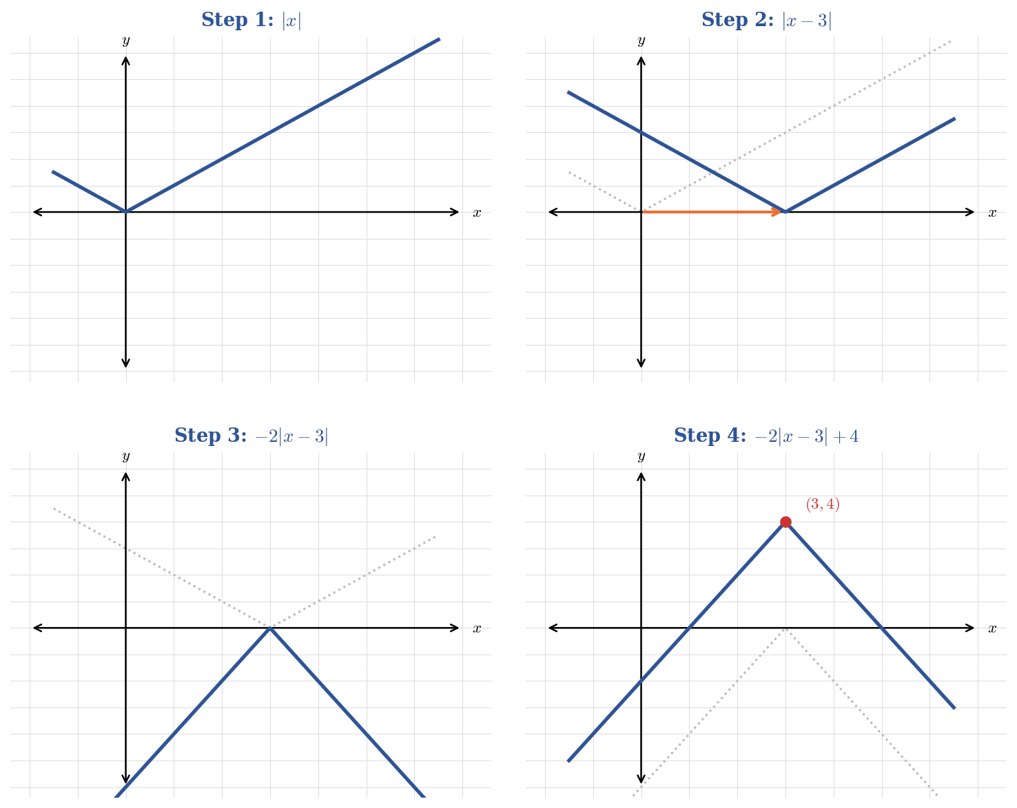
Figure 1.3.19: Building \(g(x) = -2|x - 3| + 4\) from \(f(x) = |x|\) in four steps.

TipExample 1.3.20 — Drug Concentration in the Bloodstream

After a standard dose of a certain medication, the concentration \(C(t)\) (in mg/L) in a patient’s bloodstream is modeled by \(C(t) = 5\sqrt{t}\, e^{-t/4}\) for \(t \geq 0\) hours.

A second patient receives a double dose administered \(1\) hour later. Write a function \(D(t)\) for the second patient’s concentration and describe the transformations.

Solution. A “double dose” means the concentration at every moment is twice as high: multiply the output by \(2\) (vertical stretch). “Administered \(1\) hour later” means the concentration profile starts \(1\) hour later: replace \(t\) with \(t - 1\) (shift right \(1\)).

\[D(t) = 2C(t - 1) = 2 \cdot 5\sqrt{t - 1}\, e^{-(t-1)/4} = 10\sqrt{t-1}\, e^{-(t-1)/4}, \quad t \geq 1\]

The graph of \(D\) is the graph of \(C\) shifted right \(1\) unit and stretched vertically by a factor of \(2\). The peak concentration is twice as high and occurs \(1\) hour later.

1.3.6 Even and Odd Functions

Some functions have built-in symmetry that simplifies graphing and analysis. These symmetries are closely related to reflections.

NoteDefinition 1.3.21 — Even Function

A function \(f\) is even if \(f(-x) = f(x)\) for all \(x\) in its domain. The graph of an even function is symmetric about the \(y\)-axis.

NoteDefinition 1.3.22 — Odd Function

A function \(f\) is odd if \(f(-x) = -f(x)\) for all \(x\) in its domain. The graph of an odd function is symmetric about the origin (a \(180°\) rotation maps the graph onto itself).

Figure 1.3.23 illustrates both types. The parabola \(f(x) = x^2\) is even: the left half is a mirror image of the right half. The cubic \(f(x) = x^3\) is odd: rotating the graph \(180°\) about the origin produces the same curve.

Two graphs side by side. Left: f of x equals x squared labeled as even, with symmetric points at negative 1.5 and 1.5 highlighted. Right: f of x equals x cubed labeled as odd, with points at 1 comma 1 and negative 1 comma negative 1 highlighted.

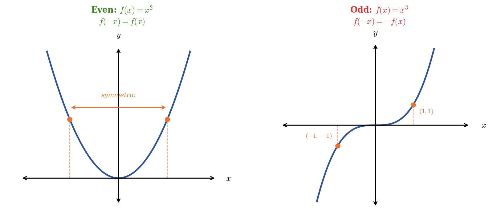
Figure 1.3.23: An even function (\(x^2\), symmetric about the \(y\)-axis) and an odd function (\(x^3\), symmetric about the origin).

TipExample 1.3.24 — Classifying Even, Odd, or Neither

Determine whether each function is even, odd, or neither.

  1. \(f(x) = x^4 - 2x^2 + 1\)
  2. \(g(x) = x^3 - x\)
  3. \(h(x) = x^2 + x\)

Solution.

The test is straightforward: compute \(f(-x)\) and compare it to \(f(x)\) and \(-f(x)\).

  1. \(f(-x) = (-x)^4 - 2(-x)^2 + 1 = x^4 - 2x^2 + 1 = f(x)\). Since \(f(-x) = f(x)\), the function is even.

  2. \(g(-x) = (-x)^3 - (-x) = -x^3 + x = -(x^3 - x) = -g(x)\). Since \(g(-x) = -g(x)\), the function is odd.

  3. \(h(-x) = (-x)^2 + (-x) = x^2 - x\). This equals neither \(h(x) = x^2 + x\) nor \(-h(x) = -x^2 - x\). The function is neither even nor odd.

TipExample 1.3.25 — Interpreting Symmetry in Context

An economist models a company’s profit as a function of how far its price deviates from the optimal price point. Let \(x\) represent the deviation (in dollars) from the optimal price, and let \(P(x) = -0.5x^2 + 200\) model the weekly profit (in thousands of dollars).

  1. Show that \(P\) is an even function.
  2. Interpret the symmetry in business terms.

Solution.

  1. \(P(-x) = -0.5(-x)^2 + 200 = -0.5x^2 + 200 = P(x)\). Since \(P(-x) = P(x)\), the function is even.

  2. The symmetry means that overpricing and underpricing by the same amount produce equal losses in profit. Charging $10 too much has the same impact on profit as charging $10 too little. The maximum profit of $200{,}000 per week occurs at the optimal price (\(x = 0\)), and any deviation — in either direction — reduces profit by the same amount.

1.3.7 Summary

  • Parent functions (\(x\), \(x^2\), \(x^3\), \(\sqrt{x}\), \(|x|\), \(1/x\)) are the building blocks from which other functions are constructed through transformations.
  • Vertical shifts: \(f(x) + k\) moves up; \(f(x) - k\) moves down.
  • Horizontal shifts: \(f(x - h)\) moves right; \(f(x + h)\) moves left. Note the opposite sign.
  • Reflections: \(-f(x)\) reflects across the \(x\)-axis; \(f(-x)\) reflects across the \(y\)-axis.
  • Vertical stretch/compression: \(a \cdot f(x)\) stretches if \(a > 1\), compresses if \(0 < a < 1\).
  • Horizontal stretch/compression: \(f(bx)\) compresses horizontally if \(b > 1\), stretches if \(0 < b < 1\).
  • When combining transformations, work inside out: horizontal changes first, then vertical changes.
  • A function is even if \(f(-x) = f(x)\) (symmetric about the \(y\)-axis) and odd if \(f(-x) = -f(x)\) (symmetric about the origin).

1.4 Building New Functions: Combinations and Composition

This section is under development.

1.5 Reversing the Process: Inverse Functions

This section is under development.

1.6 Format Preview Section

This is only a preview section to delete later. The boxes below are style previews for each environment type.

1.6.1 Sample Subsection

Some introductory text before the first box…

ImportantProblem-Solving Strategy 1.1.1 — Identifying Functions

To determine whether a relationship is a function, check that each input has exactly one output. You can use the vertical line test on a graph: if any vertical line crosses the graph more than once, it is not a function.

More text between boxes…

NoteDefinition 1.1.2 — Function

A function \(f\) from a set \(A\) to a set \(B\) is a rule that assigns to each element \(x\) in \(A\) exactly one element \(f(x)\) in \(B\). The set \(A\) is the domain and the set \(B\) is the codomain.

More text…

NoteTheorem 1.1.3 — Vertical Line Test

A curve in the \(xy\)-plane is the graph of a function of \(x\) if and only if no vertical line intersects the curve more than once.

More text…

NoteCorollary 1.1.4 — Circle Is Not a Function

A circle centered at the origin, \(x^2 + y^2 = r^2\), is not the graph of a function because vertical lines through the interior cross the circle at two points.

More text…

TipExample 1.1.5 — Evaluating a Function

Determine whether each relation is a function:

  1. \(y = x^2 + 1\)
  2. \(x^2 + y^2 = 4\)

Solution.

  1. For every input \(x\), there is exactly one output \(y = x^2 + 1\). This is a function.
  2. Solving for \(y\) gives \(y = \pm\sqrt{4 - x^2}\), which yields two outputs. This is not a function.
WarningCheckpoint 1.1.6

Is the relation \(y = \sqrt{x - 3}\) a function? What is its domain?

More text…

TipExample 1.1.7 — Finding the Domain

Find the domain of \(f(x) = \frac{1}{x - 2}\).

Solution. The function is undefined when the denominator equals zero, i.e., when \(x = 2\). Therefore the domain is \((-\infty, 2) \cup (2, \infty)\).

WarningCheckpoint 1.1.8

Find the domain of \(g(x) = \sqrt{5 - x}\).